Analysis of community composition

Abstract

This notebook takes formatted 16S rRNA amplicon counts and plots and analyzes them in different ways to look at community composition

1 Setup

Libraries and global variables

library(tidyverse)
library(here)
library(fs)
library(fishualize)
library(Polychrome)
library(withr)
library(scales)
library(patchwork)

source(here::here("R", "utils_generic.R"))

Set up some directories

data_raw <- here::here("_data_raw", "illumina_v3v4")

# make processed data directory if it doesn't exist
data <- here::here("data", "illumina_v3v4")
figs <- here::here("figs", "illumina_v3v4")

fs::dir_create(data)
fs::dir_create(figs)

1.1 Some functions

myarplot <- function(.data){
  cil <- unique(.data$predator_history)
  bac <- unique(.data$prey_history)
  
  mytitle <- case_when(cil == "anc"  & bac == "anc" ~ "anc bac + anc cil",
                       cil == "anc"  & bac == "evo" ~ "evo bac + anc cil",
                       cil == "evo"  & bac == "anc" ~ "anc bac + evo cil",
                       cil == "evo"  & bac == "evo" ~ "evo bac + evo cil",
                       cil == "nopredator" & bac == "anc" ~ "anc bac",
                       cil == "nopredator" & bac == "evo" ~ "evo bac",
                       #cil == "nopredator" & bac == "evo" ~ "starting anc bac",
                       #cil == "nopredator" & bac == "evo" ~ "starting evo bac"
  )
  
  ggplot(.data) +
    geom_area(aes(x=time_days, y=f, fill=strainID),
              color="black", size=0.1) +
    facet_wrap( ~ replicate, strip.position = "bottom") +
    scale_fill_manual(values = hambi_colors) + 
    scale_y_continuous(limits = c(0,1), expand = c(0, 0), labels = scales::percent) +
    scale_x_continuous(limits = c(4,60), breaks = c(20, 40, 60)) +
    labs(x="", y="", fill="", title=mytitle) + 
    theme_bw() + 
    myartheme()
  
}

myartheme <- function(...){
  theme(
    panel.spacing.x = unit(0.05,"line"),
    strip.placement = 'outside',
    strip.background.x = element_blank(),
    panel.grid = element_blank(),
    panel.border = element_blank(),
    panel.background = element_blank(),
    #axis.text.x = element_blank(),
    axis.line.x = element_line(color = "black"),
    axis.line.y = element_line(color = "black"),
    legend.title = element_blank(),
    legend.background = element_blank(),
    legend.key = element_blank(),
    ...)
}

strain.order <- c("HAMBI_2443", "HAMBI_3031", "HAMBI_1988", "HAMBI_3237", "HAMBI_0262", 
                  "HAMBI_2159", "HAMBI_1842", "HAMBI_2164", "HAMBI_0006", "HAMBI_0097", 
                  "HAMBI_2494", "HAMBI_1299", "HAMBI_2160", "HAMBI_1279", "HAMBI_2792", 
                  "HAMBI_1896", "HAMBI_0105", "HAMBI_0403", "HAMBI_1977", "HAMBI_1923", 
                  "HAMBI_2659", "HAMBI_1292", "HAMBI_1972", "HAMBI_1287")

Read data

counts <- read_tsv(here::here(data, "species_counts.tsv"))
metadf <- read_rds(here::here("data", "shared", "metadata_formatted.rds"))

counts_f <- left_join(metadf, counts) %>% 
  group_by(sample) %>% 
  mutate(f=count/sum(count)) %>%  
  ungroup() %>% 
  filter(!is.na(strainID))

2 Plot Community Composition

community composition of the initial conditions

pinit <- counts_f %>% 
  mutate(strainID=factor(strainID, levels=strain.order)) %>% 
  filter(str_detect(condition_prey_pred, "inoculum")) %>% 
  ggplot() + 
  geom_bar(aes(y = f, x=replicate, fill = strainID),
           color="black", size=0.25, stat="identity") +
  facet_grid(~ prey_history, scales="free_x") +
  scale_fill_manual(values = hambi_colors) + 
  scale_y_continuous(limits = c(0,1), expand = c(0, 0), labels = scales::percent) +
  labs(x="", y="% abundance", fill="", title="Community composition in starting inocula") + 
  theme_bw() + 
  myartheme()

Warning: Using `size` aesthetic for lines was deprecated in ggplot2 3.4.0.
ℹ Please use `linewidth` instead.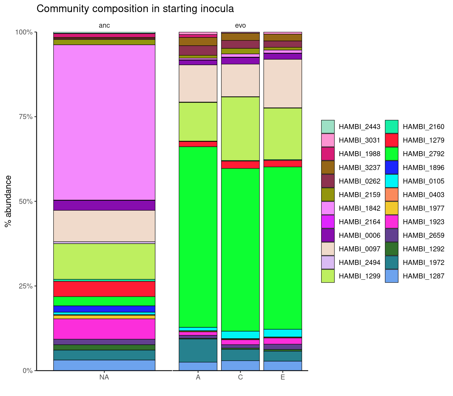

pinit

Figure 1: Community composition of the inoculae used to start the experiment

Plot community compositions during the experiment

phi <- counts_f %>% 
  mutate(strainID=factor(strainID, levels=strain.order),
         time_days = as.numeric(as.character(time_days))) %>% 
  filter(!is.na(time_days)) %>% 
  group_by(prey_history, predator_history) %>% 
  group_split() %>% 
  map(myarplot) %>% 
  wrap_plots(., ncol = 3) +
  plot_layout(guides = 'collect') +
  plot_annotation(tag_levels = 'A') & 
  theme(legend.position = 'bottom')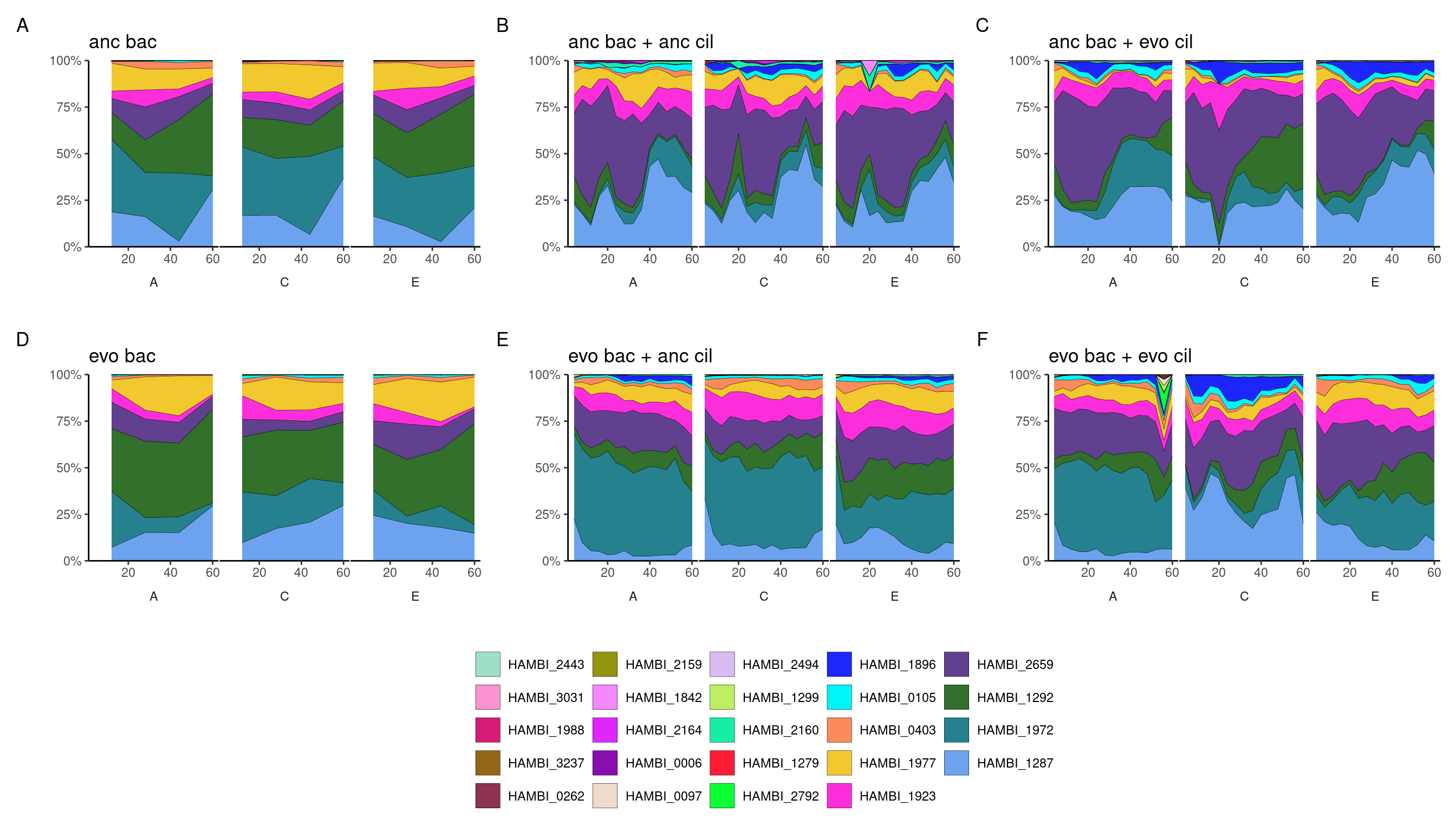

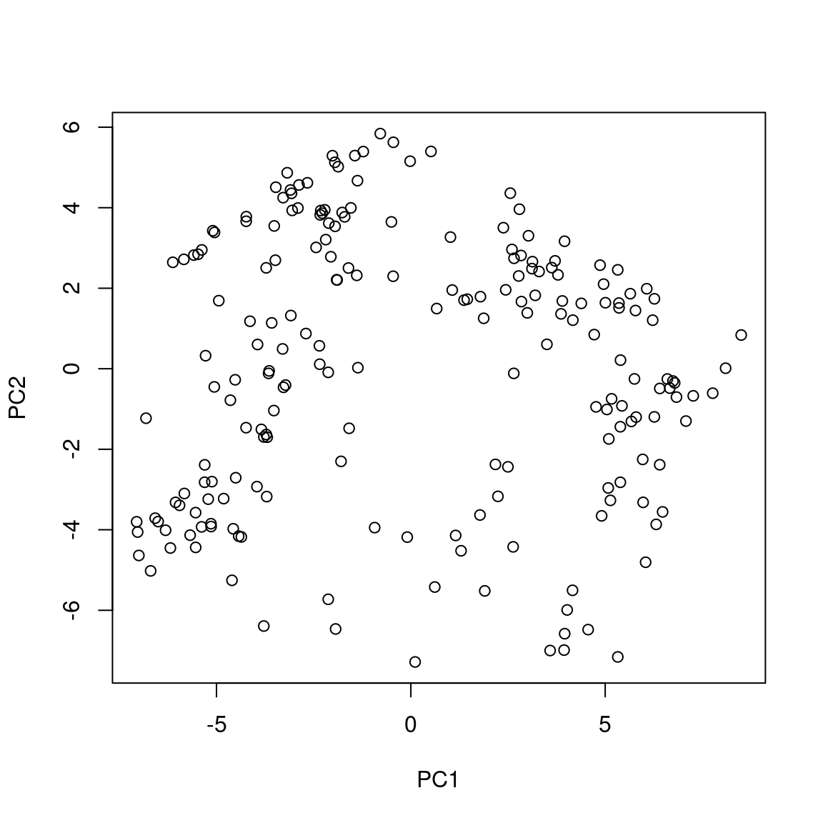
phi

Figure 2: Community composition temporal trajectories during the experiment

3 Ordination of community composition

Need some additional libraries here

library(compositions)
library(zCompositions)
library(vegan)
library(ape)
library(corrr)
library(ggrepel)

3.1 Transform data

zCompositions has problems with species with < 2 observations so we need to filter these out

lowstrains <- counts_f %>% 
  filter(!str_detect(condition_prey_pred, "inoculum")) %>% 
  filter(!is.na(count)) %>% 
  group_by(strainID) %>% 
  summarize(n_samples = n(),
            n_gt0 = sum(count > 0),
            p_gt0 = n_gt0 / n_samples) %>% 
  ungroup()

Here we remove strains present in < 50 samples across transfer categories and present in < 20 samples in at least 2/3 transfer categories

lowstrainsv <- c(
  "HAMBI_0097",
  "HAMBI_0262",
  "HAMBI_1842",
  "HAMBI_1988",
  "HAMBI_2443",
  "HAMBI_2792",
  "HAMBI_3031",
  "HAMBI_3237"
)

transform to matrix

mymat <- counts_f %>% 
  filter(!is.na(count)) %>% 
  filter(strainID %nin% lowstrainsv) %>% 
  filter(!str_detect(condition_prey_pred, "inoculum")) %>% 
  dplyr::select(sample, strainID, count) %>% 
  # important to arrange by sample as this makes some later joins easier
  arrange(sample) %>% 
  pivot_wider(names_from = "strainID", values_from = "count") %>% 
  column_to_rownames(var = "sample") %>% 
  data.frame()

3.2 Replace zeros

Compositional analysis with the centered log-ratio can’t handle zero values. Some people just replace them with a pseudocount. Another way is to impute them based on various different strategies.

Literature:

• A field guide for the compositional analysis of any-omics data
  • Supplemental material
• zCompositions — R package for multivariate imputation of left-censored data under a compositional approach

Here we will uses a Geometric Bayesian-multiplicative replacement strategy that preserves the ratios between the non-zero components. The “prop” option returns relative abundances.

set.seed(12378)
comp <- zCompositions::cmultRepl(mymat, method = "GBM", output = "prop")

No. adjusted imputations:  77 

3.3 Calculate Bray-curtis dissimilarity

set.seed(12353)
bray_dist      <- vegan::vegdist(comp, method = "bray")
pcoa_ord_bray  <- ape::pcoa(bray_dist)

3.4 Calculate with Aitchison distance

Aitchison distance is the Euclidean distance of the centered log-ratio transform (clr). This distance (unlike Euclidean distance on read counts) has scale invariance, perturbation invariance, permutation invariance and sub-compositional dominance.

set.seed(12354)
balclr     <- compositions::clr(comp)
aitc_dist  <- vegan::vegdist(balclr, method = "euclidean")

3.5 Compare Aitchison distance with CLR

When the Aitchison distance is used in Principle co-ordinate Analysis (PCoA) it is equivalent to standard Principle Component Analyis (PCA) on the clr transformed data

set.seed(12355)
pcoa_ord_aitc  <- ape::pcoa(aitc_dist)
pca_ord_aitc   <- prcomp(balclr)

For example, these ordinations are the same, just that Axis2 is the mirrorimage between. Since the rotation is arbitrary this does not matter.

plot(pcoa_ord_aitc$vectors)

Figure 3: Plot of Principal Coordinate Analysis (PCoA) done in the Aitchison geometry of the simplex (i.e. PCoA on the euclidean distance of the centered log-ratio transform species compositions).

plot(pca_ord_aitc$x)

Figure 4: Plot of Principal Component Analysis (PCA) done in the Aitchison geometry of the simplex (i.e. PCA on the centered log-ratio transform species compositions). Notice that the PCoA using the euclidean distance of centered log-ratio transformed species frequencies is equivalent to the PCA directly using clr-transformed values in Figure 3.

3.6 Environment vectors

left_join with metadata

pca2plot <- data.frame(pca_ord_aitc$x) %>% 
  rownames_to_column(var = "sample") %>% 
  left_join(metadf) %>% 
  arrange(sample) %>% 
  mutate(expcombo=interaction(condition_prey_pred, time_days, sep = "_"))

About 85% of variance explained in first 5 PCs

pca_ord_aitc_importance <- as.data.frame(summary(pca_ord_aitc)$importance) %>% 
  rownames_to_column(var = "parameter")

pca_ord_aitc_importance

Environmental/experimental variables associated with ordinatoion

ef <-
  envfit(
    pca_ord_aitc ~ prey_history + predator_history + ciliates_ml + time_days,
    data = semi_join(metadf, dplyr::select(pca2plot, sample)),
    na.rm = T,
    choices = c(1, 2)
  )

biplot(pca_ord_aitc, choices=c(1,2), labSize=0)
plot(ef)

Figure 5: Environmental vectors plotted onto ordination in Figure 4

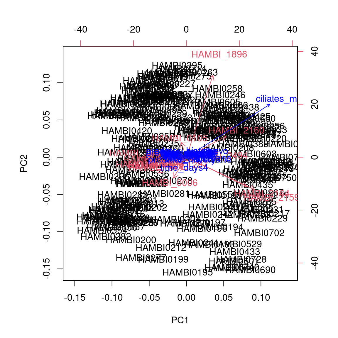
3.6.1 Significance of the environmental covariates

ef

***VECTORS

                PC1     PC2     r2 Pr(>r)    
ciliates_ml 0.84491 0.53492 0.1262  0.001 ***
---
Signif. codes:  0 '***' 0.001 '**' 0.01 '*' 0.05 '.' 0.1 ' ' 1
Permutation: free
Number of permutations: 999

***FACTORS:

Centroids:
                        PC1     PC2
prey_historyanc      4.3571 -0.5277
prey_historyevo     -3.0257  1.4454
predator_historyanc  1.1182 -1.1211
predator_historyevo  0.2132  2.0388
time_days4          -0.8610 -4.2785
time_days8           0.8755 -1.0156
time_days12          1.1134  0.1314
time_days16          1.2332  0.0357
time_days20         -0.0521  0.3658
time_days24          1.8596  1.4475
time_days28          1.5366  1.0170
time_days32          0.4066  0.7041
time_days36          0.9413  1.1857
time_days40          0.4137  1.0675
time_days44          0.4505  1.2408
time_days48          0.2291  1.2173
time_days52          0.9245  1.6736
time_days56          0.8231  0.6831
time_days60          0.0920  1.4073

Goodness of fit:
                     r2 Pr(>r)    
prey_history     0.5357  0.001 ***
predator_history 0.0991  0.001 ***
time_days        0.0911  0.246    
---
Signif. codes:  0 '***' 0.001 '**' 0.01 '*' 0.05 '.' 0.1 ' ' 1
Permutation: free
Number of permutations: 999

24 observations deleted due to missingness

con_scrs <- as.data.frame(scores(ef, display = "vectors")) %>%
  rownames_to_column(var = "var") %>% tibble()

fct_scrs <- as.data.frame(scores(ef, display = "factors")) %>% 
  rownames_to_column(var = "var") %>%  tibble()

scale_factor <- 15

3.6.2 Plot with prey history highlighted

ppca <- ggplot(pca2plot) +
  geom_point(aes(
    x = PC1,
    y = PC2,
    color = prey_history,
    shape = predator_history), size=3 ) +
  geom_segment(data = con_scrs,
               aes(x = 0, xend = PC1*scale_factor, y = 0, yend = PC2*scale_factor),
               arrow = arrow(length = unit(0.25, "cm")), colour = "black") +
  geom_text_repel(data = con_scrs, aes(x = PC1*scale_factor, y = PC2*scale_factor, label = var),
                  size = 3) +
  labs(x = paste0("PC1 (", round(pca_ord_aitc_importance[2,2]*100, 1),"%)"), 
       y = paste0("PC2 (", round(pca_ord_aitc_importance[2,3]*100, 1),"%)")) +
  stat_ellipse(aes(x = PC1, y = PC2, color = prey_history)) + 
  coord_fixed() +
  scale_color_manual(values = c("#88CCEE", "#CC6677")) +
  scale_shape_manual(values = c(1, 0, 15)) +
  theme_bw() +
  theme(
    panel.grid.major = element_blank(),
    panel.grid.minor = element_blank(),
    panel.background = element_blank(),
  )

Figure 6: Plot of principal component analysis (PCA) done in the Aitchison geometry of the simplex (i.e. centered log-ratio transform species compositions). Color shows evolutionary history of the prey and shape shows evolutionary history of the predator. 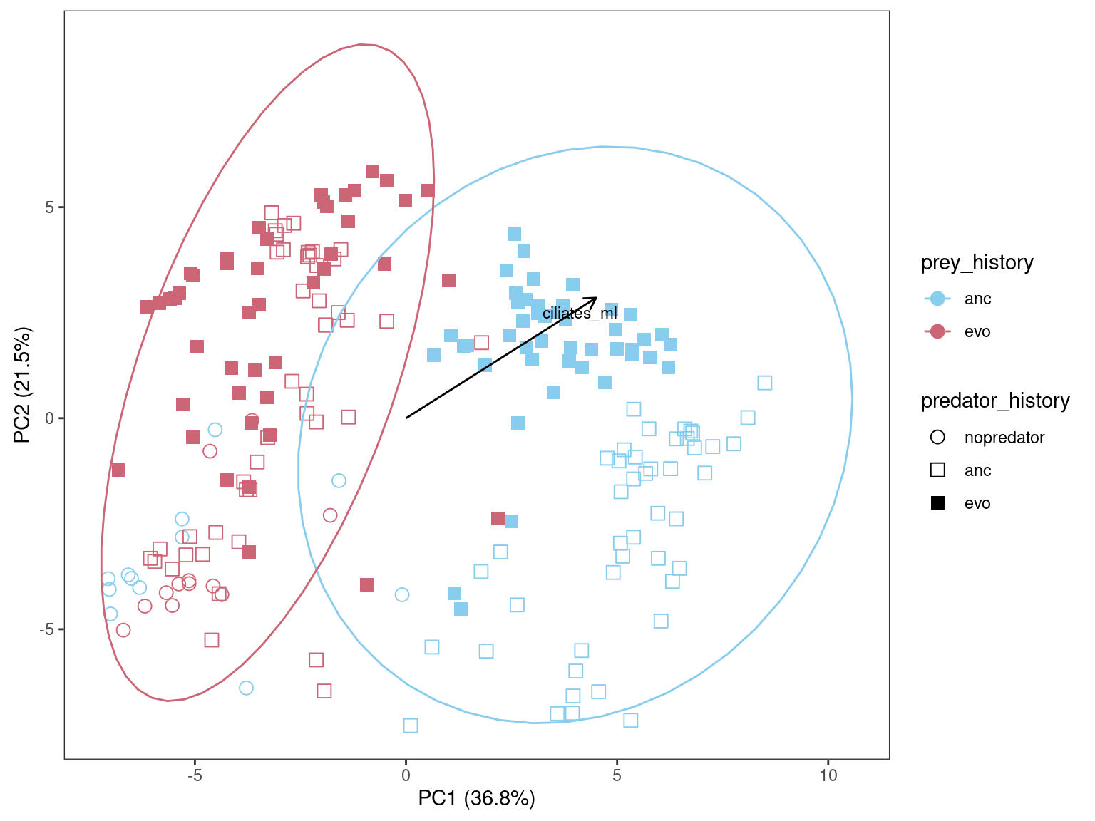Arrows and ellipses depict statistically significant (P < 0.05) experimental variables (continuous and categorical, resp) fit to the ordination axes via regression (vegan::envfit) and projected onto the ordination plot. Significance is assessed by permutation.

3.6.3 Plot with predator history highlighted

ggplot(pca2plot) +
  geom_point(aes(
    x = PC1,
    y = PC2,
    color = predator_history,
    shape = prey_history), size=3 ) +
  geom_segment(data = con_scrs,
               aes(x = 0, xend = PC1*scale_factor, y = 0, yend = PC2*scale_factor),
               arrow = arrow(length = unit(0.25, "cm")), colour = "black") +
  geom_text_repel(data = con_scrs, aes(x = PC1*scale_factor, y = PC2*scale_factor, label = var),
                  size = 3) +
  labs(x = paste0("PC1 (", round(pca_ord_aitc_importance[2,2]*100, 1),"%)"), 
       y = paste0("PC2 (", round(pca_ord_aitc_importance[2,3]*100, 1),"%)")) +
  stat_ellipse(aes(x = PC1, y = PC2, color = predator_history)) + 
  coord_fixed() +
  theme_bw() +
  theme(
    panel.grid.major = element_blank(),
    panel.grid.minor = element_blank(),
    panel.background = element_blank(),
  )

Figure 7: As in Figure 6 but with predator evolutionary history highlighted in color.

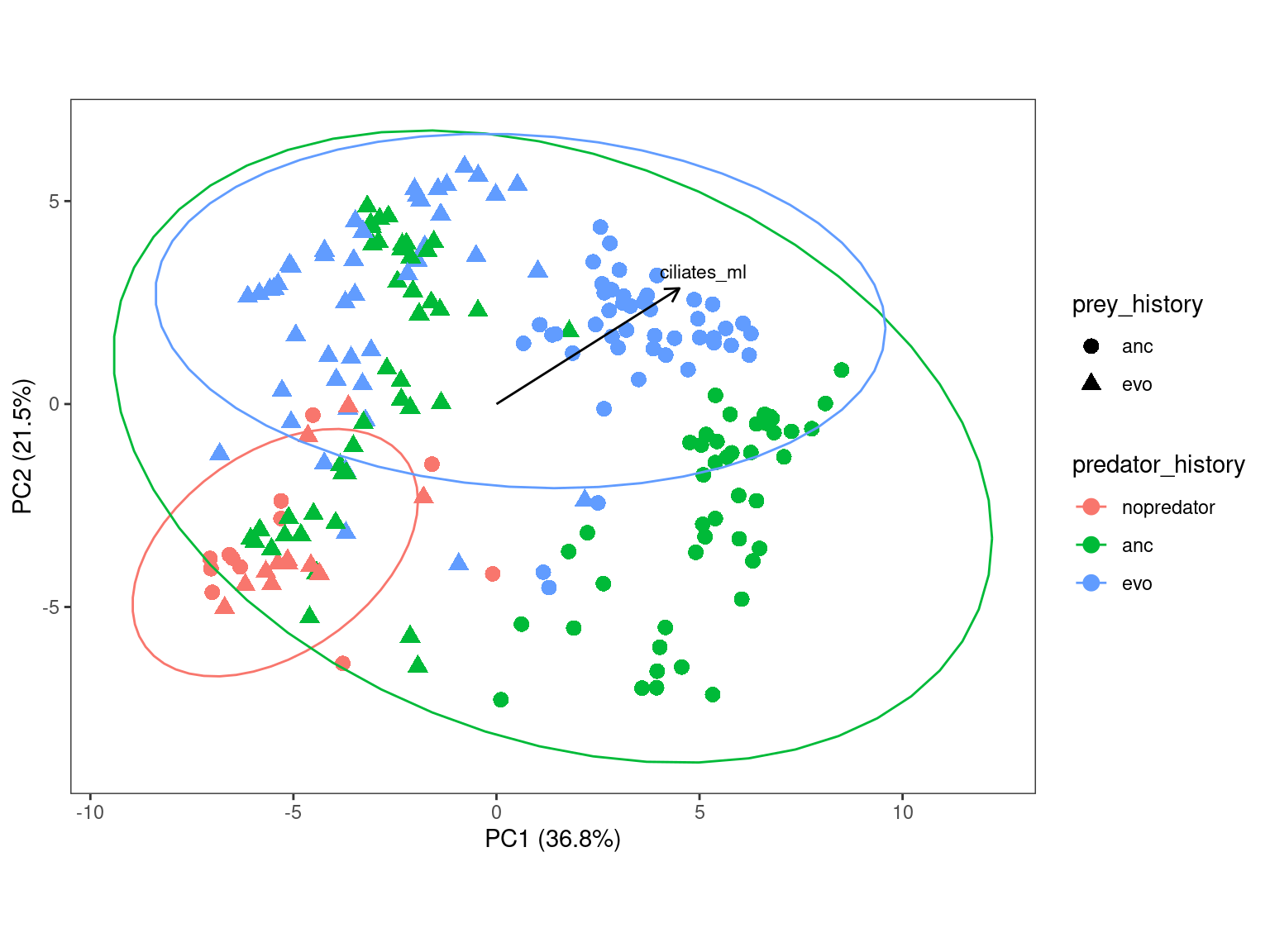
The evolved predator seems to “tighten” up the variation and make samplles with ancestral prey “look” more like the samples with evolved prey

3.6.4 PERMANOVA

PERMANOVA suggests significant effect of predator and prey evolutionary history

set.seed(45781)
adonis2(aitc_dist ~ pca2plot$prey_history + pca2plot$predator_history,
       permutations = 1e3)

Check for homogeneity of variance between these two categories. Suggests that they are different although maybe not by very much…

set.seed(45782)
bdprey <- betadisper(aitc_dist, pca2plot$prey_history)
permutest(bdprey)

Permutation test for homogeneity of multivariate dispersions
Permutation: free
Number of permutations: 999

Response: Distances
           Df Sum Sq Mean Sq      F N.Perm Pr(>F)   
Groups      1  38.61  38.613 9.4672    999  0.002 **
Residuals 202 823.88   4.079                        
---
Signif. codes:  0 '***' 0.001 '**' 0.01 '*' 0.05 '.' 0.1 ' ' 1

set.seed(45783)
bdpred <- betadisper(aitc_dist, pca2plot$predator_history)
permutest(bdpred)

Permutation test for homogeneity of multivariate dispersions
Permutation: free
Number of permutations: 999

Response: Distances
           Df Sum Sq Mean Sq     F N.Perm Pr(>F)    
Groups      2 136.53  68.263 34.83    999  0.001 ***
Residuals 201 393.94   1.960                        
---
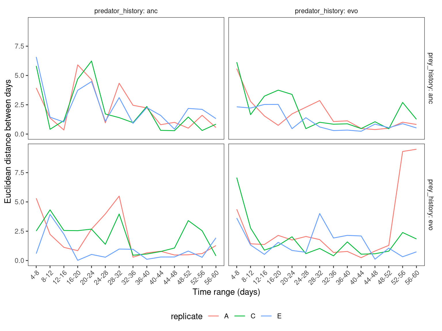
Signif. codes:  0 '***' 0.001 '**' 0.01 '*' 0.05 '.' 0.1 ' ' 1

3.7 Geometric analysis of temporal trajectories in PCA

Function to calculate euclidean distance between points

euclidean_dist <- function(x1, x2, y1, y2){
  sqrt((x1 - x2)^2 + (y1 - y2)^2)
}

eucdist <- pca2plot %>% 
  filter(prey_history != "none") %>%
  filter(predator_history != "nopredator") %>% 
  dplyr::select(PC1, PC2, replicate, prey_history, predator_history, time_days) %>% 
  arrange(replicate, prey_history, predator_history, time_days) %>% 
  group_by(replicate, prey_history, predator_history) %>% 
  mutate(d = euclidean_dist(PC1, lag(PC1), PC2, lag(PC2)),
         range = paste0(lag(time_days),"-",time_days)) %>%
  mutate(range = forcats::fct_reorder(range, as.numeric(as.character((time_days))))) %>%
  filter(range != "NA-4")

write_tsv(eucdist, here::here(data, "aitchison_pca_distances.tsv"))

ggplot(eucdist) +
  geom_line(aes(x = range, y = d, color = replicate, group=replicate)) +
  labs(x = "Time range (days)", y = "Euclidean distance between days") +
  scale_x_discrete(guide = guide_axis(angle = 45)) +
  facet_grid(prey_history ~ predator_history, labeller = label_both, scales = "free_x") +
  theme_bw() +
  theme(
    legend.position = "bottom",
    strip.placement = 'outside',
    strip.background = element_blank(),
    panel.grid = element_blank())

Figure 8: Geometric analysis of community trajectories based on PCA. Segment lengths between consecutive sampling days in the two PCA dimensions were calculated and plotted chronologically for each biological replicate in each treatment combination. As sampling intervals were of equal duration (except day 16 - 24), segment length represents relative speed of compositional change.