Formatting growth curves from Synergy H1

Abstract

The ancestral (streptomycin sensitive) and evolved (streptomycin resistant) forms of HAMBI_1287 and HAMBI_1977 were grown on Biolog Ecoplates. These are basically a set of 32 different carbon compounds in 3 replicated sets on a 96 well plate. Microbial species or communities grown on these carbon compounds respire and reduce some dye to a purple color which is then measured on a Synergy H1 multimode microplate reader.

1 Setup

1.1 Libraries

library(here)
library(tidyverse)
library(readxl)
library(stringr)
library(lubridate)
library(fs)
library(ggforce)
library(slider)
source(here::here("R", "utils_gcurves.R"))

1.2 Global variables

data_raw <- here::here("_data_raw", "biolog_ecoplates")
data <- here::here("data", "biolog_ecoplates")

# make processed data directory if it doesn't exist
fs::dir_create(data)

2 Tidying growth curves from Synergy H1 multimode microplate reader

2.1 Read growth curves

plate01 <- readxl::read_xlsx(here::here(data_raw, "biolog_ecoplate_1287A", "1287A_raw_data.xlsx"), sheet = 3, skip = 1) %>% 
  # set interval start to be first cell and make all intervals relative to that
  # use time_length to just create an hours variable of type numeric
  mutate(seconds = lubridate::time_length(lubridate::interval(Time[1], Time), unit = "second")) %>% 
  tidyr::pivot_longer(c(-seconds, -Time), names_to = "well", values_to = "OD600") %>%
  mutate(hours = lubridate::time_length(seconds, unit = "hours")) %>% 
  # converting the well format so it matches the samplesheet
  mutate(well = paste0(str_extract(well, "^[A-H]"), str_pad(str_extract(well, "\\d+"), width = 2, pad = "0", side = "left"))) %>% 
  dplyr::select(seconds, hours, well, OD600) %>% 
  # create a plate variable for later combining
  mutate(plate_name = "plate01")

plate02 <- readxl::read_xlsx(here::here(data_raw, "biolog_ecoplate_1287E_1977A", "1287E_1977A_rawdata.xlsx"), sheet = 3, skip = 1) %>% 
  # set interval start to be first cell and make all intervals relative to that
  # use time_length to just create an hours variable of type numeric
  mutate(seconds = lubridate::time_length(lubridate::interval(Time[1], Time), unit = "second")) %>% 
  tidyr::pivot_longer(c(-seconds, -Time), names_to = "well", values_to = "OD600") %>%
  mutate(hours = lubridate::time_length(seconds, unit = "hours")) %>% 
  # converting the well format so it matches the samplesheet
  mutate(well = paste0(str_extract(well, "^[A-H]"), str_pad(str_extract(well, "\\d+"), width = 2, pad = "0", side = "left"))) %>% 
  dplyr::select(seconds, hours, well, OD600) %>% 
  # create a plate variable for later combining
  mutate(plate_name = "plate02")

plate03 <- readxl::read_xlsx(here::here(data_raw, "biolog_ecoplate_1977A_1977E", "1977A_1977E_rawdata.xlsx"), sheet = 3, skip = 1) %>% 
  # set interval start to be first cell and make all intervals relative to that
  # use time_length to just create an hours variable of type numeric
  mutate(seconds = lubridate::time_length(lubridate::interval(Time[1], Time), unit = "second")) %>% 
  tidyr::pivot_longer(c(-seconds, -Time), names_to = "well", values_to = "OD600") %>%
  mutate(hours = lubridate::time_length(seconds, unit = "hours")) %>% 
  # converting the well format so it matches the samplesheet
  mutate(well = paste0(str_extract(well, "^[A-H]"), str_pad(str_extract(well, "\\d+"), width = 2, pad = "0", side = "left"))) %>% 
  dplyr::select(seconds, hours, well, OD600) %>% 
  # create a plate variable for later combining
  mutate(plate_name = "plate03")

3 Format growth curves

3.1 Read sample metadata

samplesheet01 <- readxl::read_xlsx(here::here(data_raw, "biolog_ecoplate_1287A", "samplesheet_1287A.xlsx")) %>% 
  mutate(strainID = paste0("HAMBI_", strain)) %>% 
  mutate(plate_name = "plate01")
samplesheet02 <- readxl::read_xlsx(here::here(data_raw, "biolog_ecoplate_1287E_1977A", "samplesheet_1287E_1977A.xlsx")) %>% 
  mutate(strainID = paste0("HAMBI_", strain)) %>% 
  mutate(plate_name = "plate02")
samplesheet03 <- readxl::read_xlsx(here::here(data_raw, "biolog_ecoplate_1977A_1977E", "samplesheet_1977A_1977E.xlsx")) %>% 
  mutate(strainID = paste0("HAMBI_", strain)) %>% 
  mutate(plate_name = "plate03")

3.2 Join with metadata to remove ununsed samples

ecoplate_gcurves_sm <- bind_rows(plate01, plate02, plate03) %>% 
  left_join(bind_rows(samplesheet01, samplesheet02, samplesheet03), by = join_by(well, plate_name)) %>% 
  dplyr::group_by(plate_name, well) %>% 
  dplyr::mutate(OD600_rollmean = slider::slide_dbl(OD600, mean, .before = 2, .after = 2)) %>% 
  ungroup() %>% 
  relocate(OD600_rollmean, .after = "OD600")

readr::write_tsv(ecoplate_gcurves_sm, here::here(data, "ecoplate_gcurves_smooth.tsv"))

4 Inspect growth curves

4.1 plate01 (Ancestral HAMBI_1287 ANC)

This plate contains three replicates for the ancestral form of HAMBI_1287

Figure 1: Growth curves for the first ecolog plate with the ancestral form of HAMBI_1287. X-axis is time in hours (48 hour incubation). Y axis is the absorbance scaled for each well. Blue line is smoothed with a moving average window of 9 points. Orange is non-smoothed

Figure 2: As in Figure 1 but for EVO_1287 (columns 1-8) and ANC_1977 (columns 9-12)

Figure 3: As in Figure 1 but for ANC_1977 (columns 1-4) and EVO_1977 (columns 5-12)

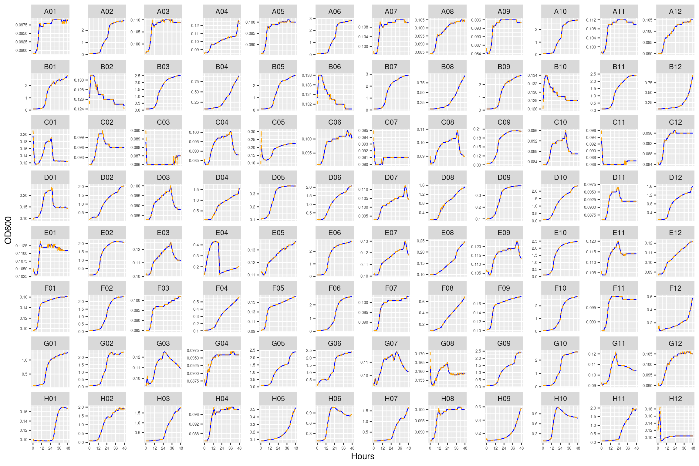
4.2 Conclusions

Growth curves all look mostly reasonable. For just a couple of the carbon substrates there are some strange features (e.g., L-asparagine for HAMBI_1977). Can proceed with the analysis.

5 Growth curve statistics

library("growthrates")

Loading required package: lattice

Loading required package: deSolve

library("DescTools")

Using the tool growthrates to estimate mu_max. I have found this works a lot better the gcplyr and is more convenient than using another tool outside of R. Nonparametric estimate growth rates by spline is very fast. Fitting to a model takes more time resources. Generally it is best to try multiple approaches and to visualize/check the data to make sure it makes sense.

ecoplate_gcurves_sm <- ecoplate_gcurves_sm %>% 
  # make uniq id
  mutate(id = paste0(plate_name, "|", well))

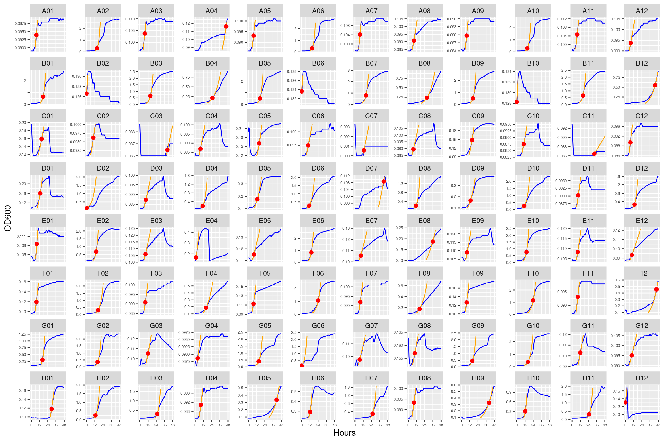
5.1 Spline based estiamte

Smoothing splines are a quick method to estimate maximum growth. The method is called nonparametric, because the growth rate is directly estimated from the smoothed data without being restricted to a specific model formula.

From growthrates documentation:

The method was inspired by an algorithm of Kahm et al. (2010), with different settings and assumptions. In the moment, spline fitting is always done with log-transformed data, assuming exponential growth at the time point of the maximum of the first derivative of the spline fit. All the hard work is done by function smooth.spline from package stats, that is highly user configurable. Normally, smoothness is automatically determined via cross-validation. This works well in many cases, whereas manual adjustment is required otherwise, e.g. by setting spar to a fixed value [0, 1] that also disables cross-validation.

5.1.1 Fit

set.seed(45278)
many_spline <- growthrates::all_splines(OD600_rollmean ~ hours | id, data = ecoplate_gcurves_sm, spar = 0.5)

readr::write_rds(many_spline, here::here(data, "spline_fits"))

5.1.2 Results

many_spline_res <- growthrates::results(many_spline)

5.1.3 Predictions

many_spline_xy <- purrr::map(many_spline@fits, \(x) data.frame(x = x@xy[1], y = x@xy[2])) %>% 
  purrr::list_rbind(names_to = "id") 

many_spline_fitted <- purrr::map(many_spline@fits, \(x) data.frame(x@FUN(x@obs$time, x@par))) %>% 
  purrr::list_rbind(names_to = "id") %>% 
  dplyr::rename(hours = time, predicted = y) %>% 
  dplyr::left_join(ecoplate_gcurves_sm, by = dplyr::join_by(id, hours)) %>% 
  dplyr::group_by(id) %>% 
  # this step makes sure we don't plot fits that go outside the range of the data
  dplyr::mutate(predicted = dplyr::if_else(dplyr::between(predicted, min(OD600_rollmean), max(OD600_rollmean)), predicted, NA_real_)) %>% 
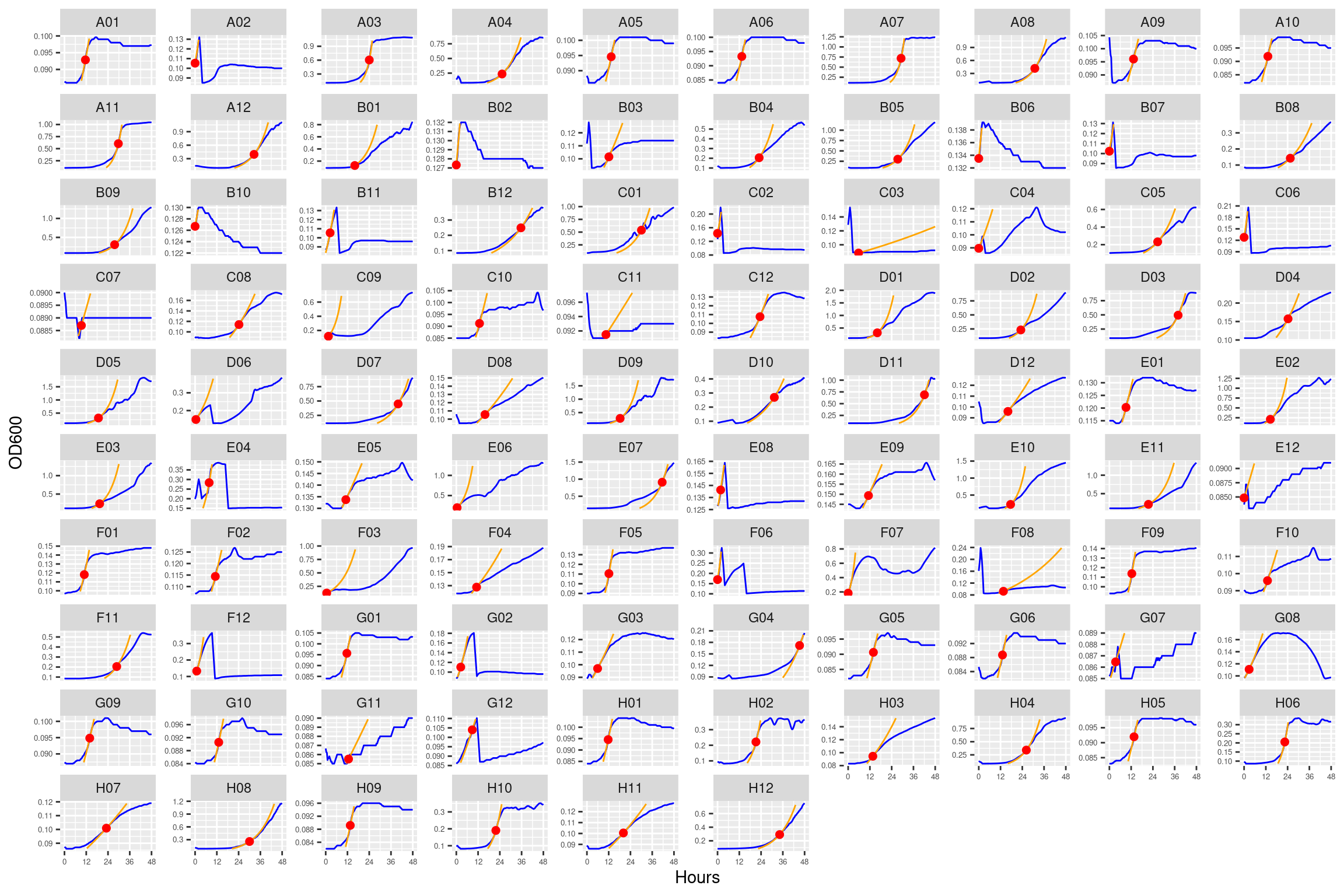
  dplyr::ungroup()

5.1.4 Plot

5.1.4.1 Plate01 (ANC_1287)

Figure 4: As in Figure 1. Blue line is smoothed with a moving average window of 5 points. Orange is slope of max predicted growth rate from the first derivative of a smoothing spline. Red dot is hours and OD600 at which maximum growth rate is reached.

5.1.4.2 Plate02 (EVO_1287 and ANC_1977)

Figure 5: As in Figure 2. Blue line is smoothed with a moving average window of 5 points. Orange is slope of max predicted growth rate from the first derivative of a smoothing spline. Red dot is hours and OD600 at which maximum growth rate is reached.

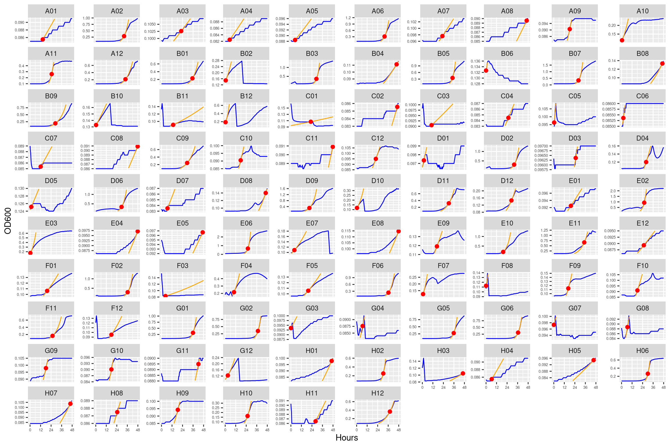
5.1.4.3 Plate03 (ANC_1977 and EVO_1977)

Figure 6: As in Figure 3. Blue line is smoothed with a moving average window of 5 points. Orange is slope of max predicted growth rate from the first derivative of a smoothing spline. Red dot is hours and OD600 at which maximum growth rate is reached.

5.2 AUC

Calculates AUC using DescTools package

many_auc_res <- ecoplate_gcurves_sm %>% 
  dplyr::summarize(auc = DescTools::AUC(hours, OD600_rollmean),
            max_od = max(OD600_rollmean),
            min_od = min(OD600_rollmean),
            .by = id) %>% 
  dplyr::left_join(dplyr::distinct(dplyr::select(ecoplate_gcurves_sm, plate_name:id)), by = join_by(id)) %>% 
  dplyr::select(-id) %>% 
  dplyr::relocate(auc, max_od, min_od, .after="strainID")

6 Write all output

readr::write_tsv(many_auc_res, here::here(data, "ecoplate_gcurve_auc_results.tsv")) 

many_spline_res %>% 
  dplyr::left_join(dplyr::distinct(dplyr::select(ecoplate_gcurves_sm, plate_name:id)), by = join_by(id)) %>% 
  dplyr::select(-id) %>% 
  dplyr::relocate(y0:r2, .after="strainID") %>% 
  readr::write_tsv(here::here(data, "ecoplate_gcurve_spline_results.tsv"))