Monoculture growth

Abstract

Growth of strains at different Streptomycin concentrations

1 Introduction

Inspect the growth of both Streptomycin-sensitive (Sens/Anc) and Streptomycin-resistant (Res/Evo) forms of Citrobacter koseri 1287 and Pseudomonas chlororaphis 1977 at different streptomycin concentrations.

##### Libraries
library(tidyverse)
library(here)
library(fs)
library(scales)
##### Global vars
data <- here::here("data", "bioscreen_strains")

2 Read

many_auc_res <- readr::read_tsv(here::here(data, "gcurve_auc_results.tsv"))
many_spline_res <- readr::read_tsv(here::here(data, "gcurve_spline_results.tsv"))
gcurves <- readr::read_tsv(here::here(data, "gcurves_formatted_thinned.tsv"))

3 Monoculture growth with streptomycin

We’ll now examine how the monoculture growth changed with respect to evolutionary history and streptomycin concentrations

3.1 Growth rates

gr_strep <- many_spline_res %>% 
  mutate(hist = str_split_i(sp_hist, "_", 1),
         sp = str_split_i(sp_hist, "_", 2)) %>% 
  summarize(ggplot2::mean_cl_boot(mumax), .by=c(sp, hist, strep_conc)) %>% 
  mutate(strep_conc = factor(strep_conc, ordered = TRUE)) %>% 
  ggplot(aes(x = strep_conc, y = y)) +
  geom_linerange(aes(ymin = ymin, ymax = ymax, color = hist)) +
  geom_line(aes(color = hist, group = hist), lty=1) +
  geom_point(aes(color = hist)) +
  labs(y = "Maximum per capita growth rate μ (hr-1)", x = "Streptomycin conc. (μg/ml)", 
       color = "Evolutionary\nhistory") +
  facet_grid(~sp) +
  scale_x_discrete(guide = guide_axis(angle = 90))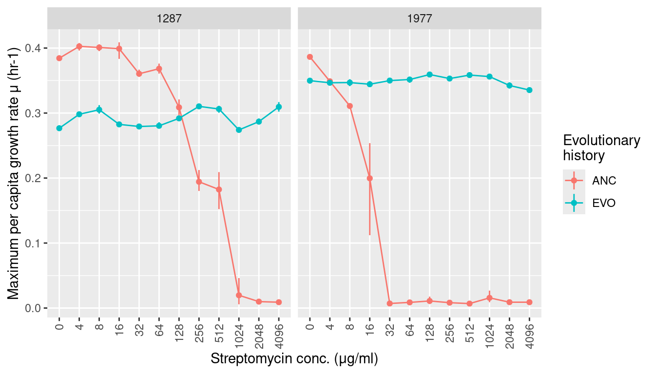

Figure 1: Maximum specific growth rate (\(\mathrm{\mu_{max}}\) in \(\mathrm{hr^{-1}}\)) for the four different bacterial species (panels) and their different evolutionary histories (colors) at different streptomycin concentrations (horizontal axis, μg/ml). Points are the mean over five biological replicates and line ranges show the 95% confidence interval from bootstraps. EVO = experimentally evolved to high streptomycin.

3.2 Maximum carrying capcaity (K, maximum observed OD)

k_strep <- many_auc_res %>% 
  mutate(hist = str_split_i(sp_hist, "_", 1),
         sp = str_split_i(sp_hist, "_", 2)) %>% 
  summarize(ggplot2::mean_cl_boot(max_od), .by=c(sp, hist, strep_conc)) %>% 
  mutate(strep_conc = factor(strep_conc, ordered = TRUE)) %>% 
  ggplot(aes(x = strep_conc, y = y)) +
  geom_linerange(aes(ymin = ymin, ymax = ymax, color = hist)) +
  geom_line(aes(color = hist, group = hist), lty=1) +
  geom_point(aes(color = hist)) +
  labs(y = "Maximum carrying capacity (K, OD units)", x = "Streptomycin conc. (μg/ml)", 
       color = "Evolutionary\nhistory") +
  facet_grid(~sp) +
  scale_x_discrete(guide = guide_axis(angle = 90))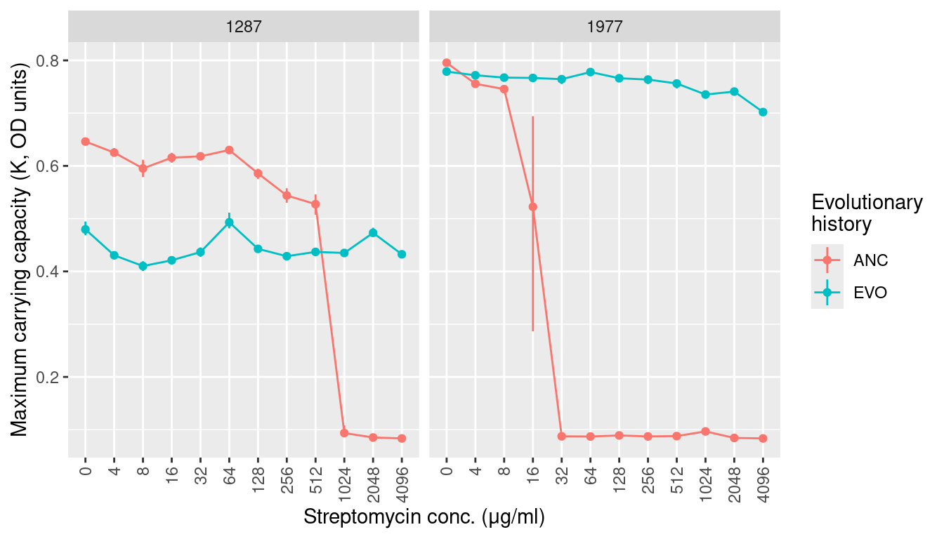

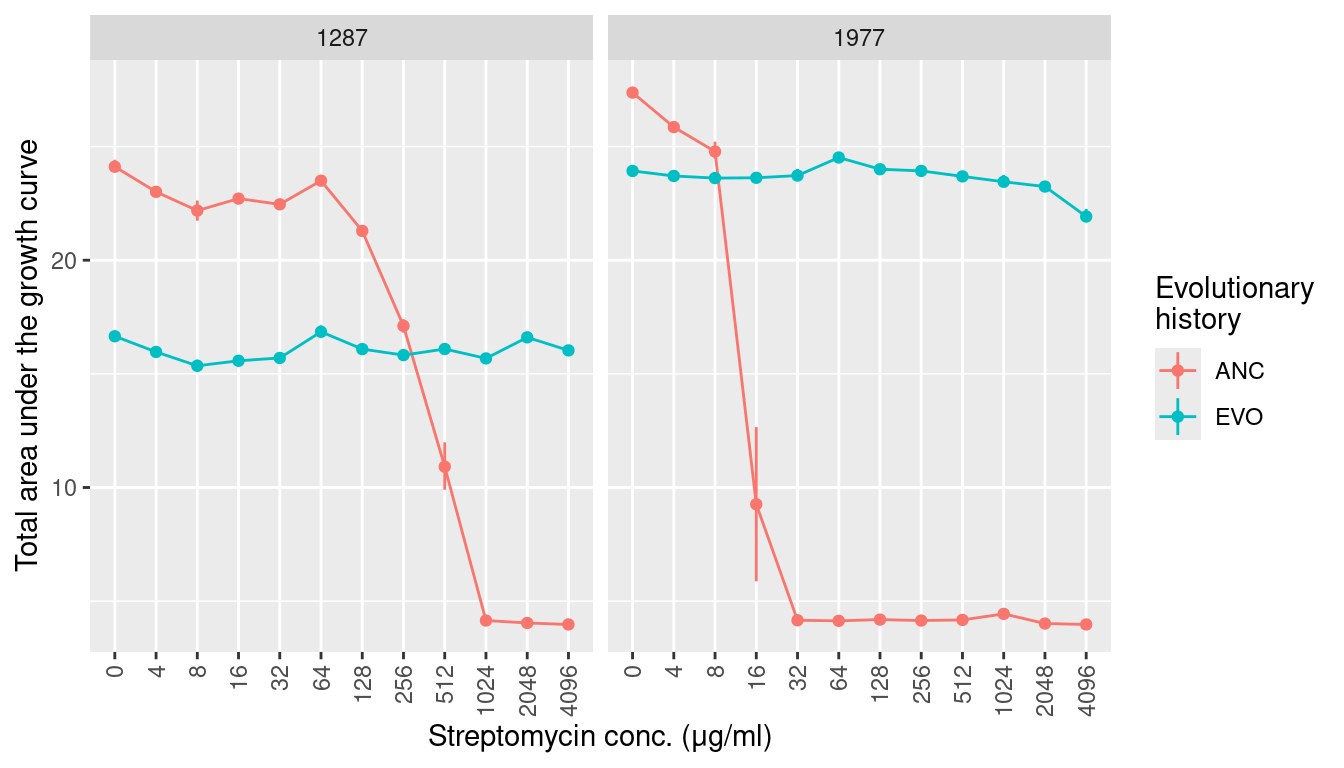
Figure 2: As in Figure 1 and Figure 2 but for maximum carrying capacity (K, maximum observed OD)

3.3 AUC (area under the growth curve)

auc_strep <- many_auc_res %>% 
  mutate(hist = str_split_i(sp_hist, "_", 1),
         sp = str_split_i(sp_hist, "_", 2)) %>% 
  summarize(ggplot2::mean_cl_boot(auc), .by=c(sp, hist, strep_conc)) %>% 
  mutate(strep_conc = factor(strep_conc, ordered = TRUE)) %>% 
  ggplot(aes(x = strep_conc, y = y)) +
  geom_linerange(aes(ymin = ymin, ymax = ymax, color = hist)) +
  geom_line(aes(color = hist, group = hist), lty=1) +
  geom_point(aes(color = hist)) +
  labs(y = "Total area under the growth curve", x = "Streptomycin conc. (μg/ml)", 
       color = "Evolutionary\nhistory") +
  facet_grid(~sp) +
  scale_x_discrete(guide = guide_axis(angle = 90))

Figure 3: Area under the growth curve for the four different bacterial species (panels) and their different evolutionary histories (colors) at different streptomycin concentrations (horizontal axis, μg/ml). Points are the mean over five biological replicates and line ranges show the 95% confidence interval from bootstraps. EVO = experimentally evolved to high streptomycin.