In the prior step we imported, smoothed, and calculated summary statistics for the species growth on the coculture plates. Here we will do some simple plots and analysis of the cocultures growth.
Show/hide code
##### Librarieslibrary(tidyverse)library(here)library(fs)library(scales)source(here::here("R", "utils_gcurves.R"))##### Global variablesdata_raw <- here::here("_data_raw", "coculture_plate")data <- here::here("data", "coculture_plate")# make processed data directory if it doesn't existfs::dir_create(data)
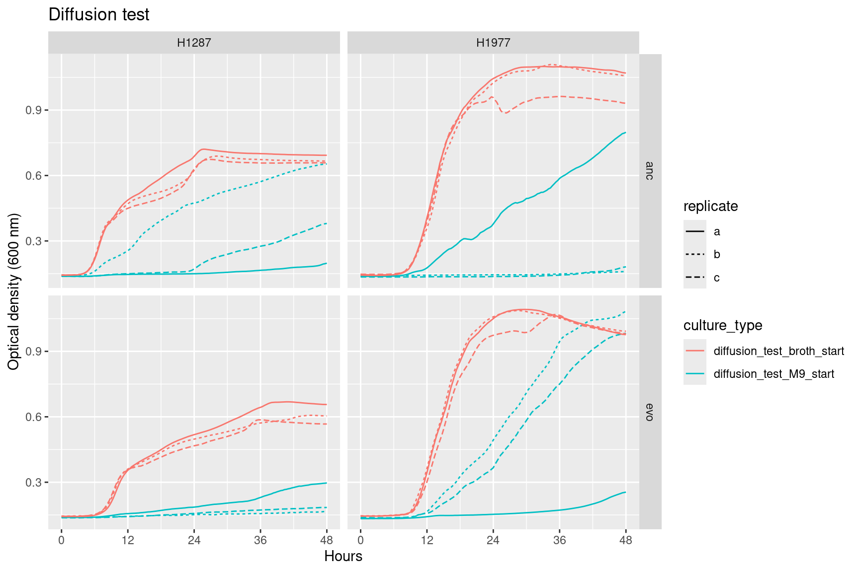
Plot the co-cultures growing on M9 compared to the control (column 1 and 3)
Show/hide code
gcurves %>%filter(str_detect(culture_type, "diffusion")) %>%filter(str_detect(strain, "NANA", negate=TRUE)) %>%ggplot() + ggplot2::geom_line(aes(x = hours, y = OD600_rollmean, lty = replicate, color = culture_type, group =interaction(well, plate_name))) + ggplot2::labs(x ="Hours", y ="OD600") + ggplot2::scale_x_continuous(breaks =seq(0, 48, 12), labels =seq(0, 48, 12)) +labs(y ="Optical density (600 nm)", x ="Hours", title ="Diffusion test") +facet_grid(evolution~strain)
Figure 1: Growth curves (OD600 over 48 hours) in monoculture for three replicates (line type) of each species (plot panel columns) and evolution status (plot panel rows). Line color indicates experimental conditions: Blue = “Double Media” which is standard inoculation into R2A growth medium with an adjacent well also containing R2A growth medium but with no inoculum. Green = diffusion test where bacteria are inoculated into M9 salts adjacent to a well containing R2A growth medium but with no inoculum. Red = diffusion test where bacteria are inoculated into R2A medium adjacent to a well containing M9 salts but with no inoculum. On the plate, column \(n=\{1\dots11\}\) is connected to column \(n+1\) with a 0.22 um membrane allowing free diffusion of resources and metabolic byproducts but not cells. These experiments were all conducted with no Streptomycin. Strain naming convention: 1287 = Citrobacter koserii 1287, 1977 = Psuedomonas chlororaphis 1977, A = Ancestral/Streptomycin sensitive, E = Evolved/Streptomycin resistant.
2.2 Monocultures and cocultures
Show/hide code
### Formatting and plotting functions# This function collects all the data from monocultures and cocultures for the selected species pair# only monoculture data from streptomycin concentrations tested in co-cultures is includedcollect_sp_pairs <-function(df, competition_pair, strep_thresh){ strainpairs <- stringr::str_split(competition_pair, "_")[[1]] df %>%mutate(streptomycin =if_else(plate_name =="plate01", 0, streptomycin)) %>%mutate(strainID =paste0(stringr::str_to_upper(stringr::str_sub(evolution, start =1, end=1)), str_extract(strain, "\\d+"))) %>%filter(strainID %in% strainpairs) %>%filter(str_detect(culture_type, "diffusion", negate = T)) %>%filter(streptomycin <= {{ strep_thresh }}) %>%filter((culture_type =="coculture"& competition_pair == {{ competition_pair}} ) | culture_type =="monoculture") %>%mutate(culture_type =factor(culture_type, levels =c("monoculture", "coculture"))) }# this function plots the output from the collect_sp_pairs functionplot_sp_pairs <-function(df, title, ncol){ straincols <-c("A1287"="orange", "E1287"="purple", "A1977"="dodgerblue", "E1977"="limegreen") ggplot2::ggplot(df) + ggplot2::geom_line(aes(x = hours, y = OD600_rollmean, color = strainID, lty = culture_type, group =interaction(well, plate_name))) + ggplot2::labs(x ="Hours", y ="OD600") + ggplot2::scale_x_continuous(breaks =seq(0, 48, 12), labels =seq(0, 48, 12)) + ggplot2::labs(y ="Optical density (600 nm), log scale", x ="Hours", title = {{title}}) + ggplot2::scale_color_manual(values = straincols) + ggplot2::scale_y_continuous(trans ="log", breaks =c(0, 0.25, 0.5, 1)) + ggplot2::facet_wrap(~streptomycin, ncol = {{ncol}}) + ggplot2::theme_bw()}
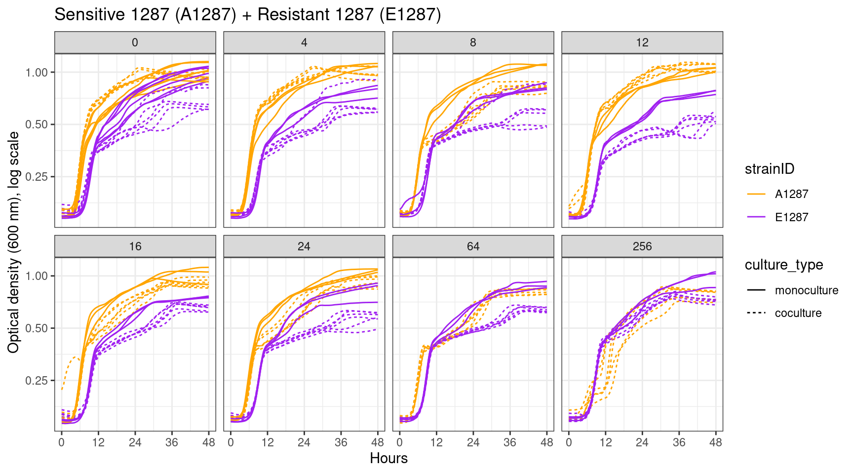
Figure 2: Growth curves (OD600 over 48 hours) of two strains in a competing pair (denoted by color and plot title). Line type denotes growth under pairwise competition (dashed line) or in monoculture. Plot panels depict the streptomycin concentration (ug/ml) under which growth was measured. Each co-culture condition was replicated six times while monoculture conditions were replicated three times. Plot panel rows depict growth in different streptomycin concentrations (ug/ml). Strain naming convention: 1287 = Citrobacter koserii 1287, 1977 = Psuedomonas chlororaphis 1977, A = Ancestral/Streptomycin sensitive, E = Evolved/Streptomycin resistant.
Important! A1977 monoculture results at 8 ug/ml streptomycin are strange, and I do not trust they are valid. The lag phase is much longer than at 12 or 16 ug/ml. I suspect this is from an experimental error and these curves should not be used. We can work to redo the measurements at 8 ug/ml
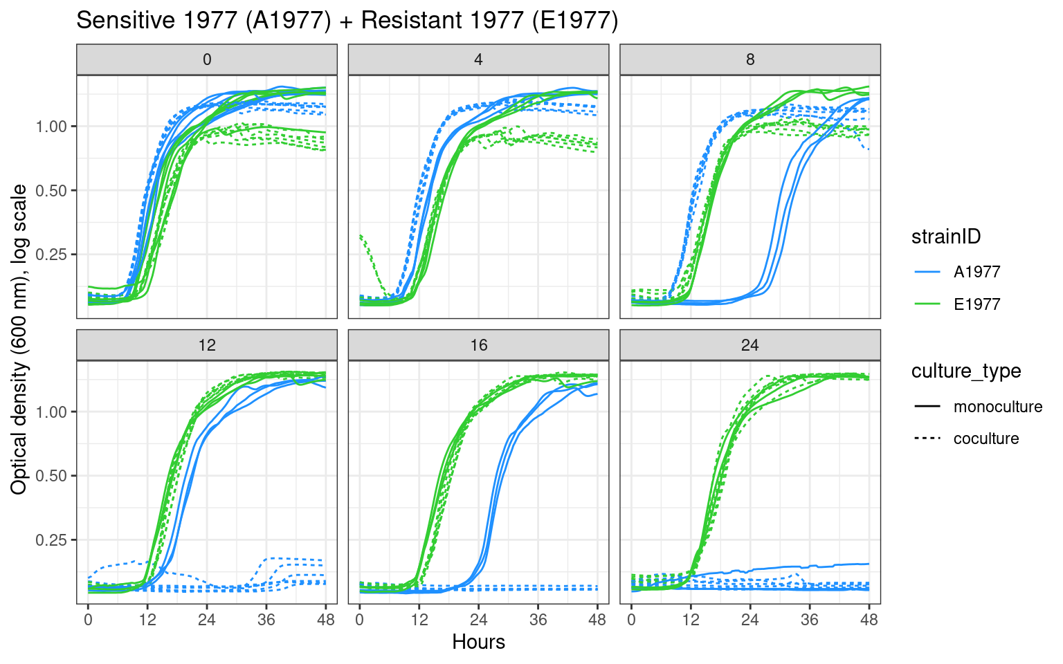
Figure 3: Growth curves (OD600 over 48 hours) of two strains in a competing pair (denoted by color and plot title). Line type denotes growth under pairwise competition (dashed line) or in monoculture. Plot panels depict the streptomycin concentration (ug/ml) under which growth was measured. Each co-culture condition was replicated six times while monoculture conditions were replicated three times. Plot panel rows depict growth in different streptomycin concentrations (ug/ml). Strain naming convention: 1287 = Citrobacter koserii 1287, 1977 = Psuedomonas chlororaphis 1977, A = Ancestral/Streptomycin sensitive, E = Evolved/Streptomycin resistant.
Important! A1977 monoculture results at 8 ug/ml streptomycin are strange, and I do not trust they are valid. The lag phase is much longer than at 12 or 16 ug/ml. I suspect this is from an experimental error and these curves should not be used. We can work to redo the measurements at 8 ug/ml
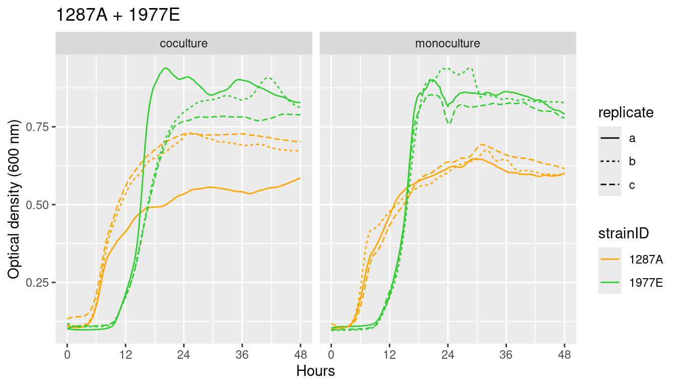
Figure 4: Growth curves (OD600 over 48 hours) of two strains in a competing pair (denoted by color and plot title). Line type denotes growth under pairwise competition (dashed line) or in monoculture. Plot panels depict the streptomycin concentration (ug/ml) under which growth was measured. Each co-culture condition was replicated six times while monoculture conditions were replicated three times. Plot panel rows depict growth in different streptomycin concentrations (ug/ml). Strain naming convention: 1287 = Citrobacter koserii 1287, 1977 = Psuedomonas chlororaphis 1977, A = Ancestral/Streptomycin sensitive, E = Evolved/Streptomycin resistant.
Important! A1977 monoculture results at 8 ug/ml streptomycin are strange, and I do not trust they are valid. The lag phase is much longer than at 12 or 16 ug/ml. I suspect this is from an experimental error and these curves should not be used. We can work to redo the measurements at 8 ug/ml
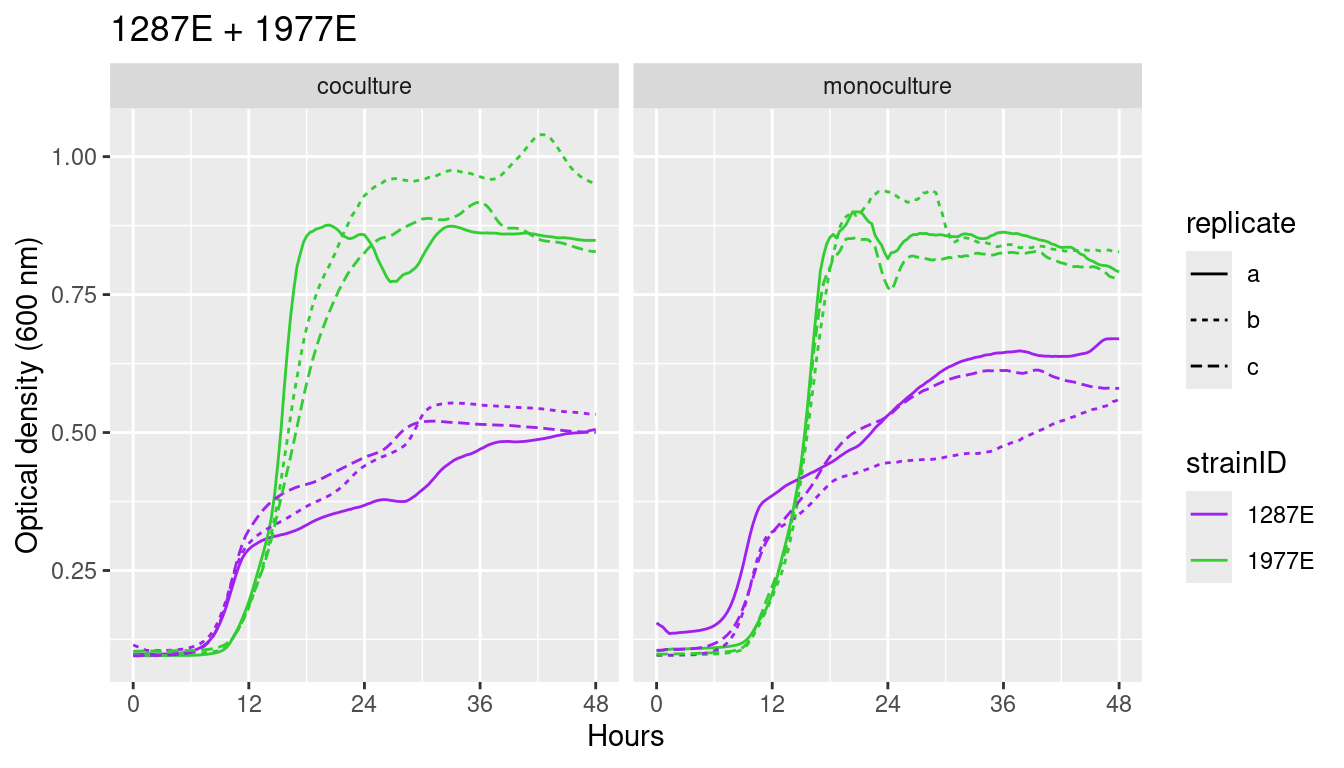
Figure 5: Growth curves (OD600 over 48 hours) of two strains in a competing pair (denoted by color and plot title). Line type denotes growth under pairwise competition (dashed line) or in monoculture. Plot panels depict the streptomycin concentration (ug/ml) under which growth was measured. Each co-culture condition was replicated six times while monoculture conditions were replicated three times. Plot panel rows depict growth in different streptomycin concentrations (ug/ml). Strain naming convention: 1287 = Citrobacter koserii 1287, 1977 = Psuedomonas chlororaphis 1977, A = Ancestral/Streptomycin sensitive, E = Evolved/Streptomycin resistant.
Figure 6: Growth curves (OD600 over 48 hours) of two strains in a competing pair (denoted by color and plot title). Line type denotes growth under pairwise competition (dashed line) or in monoculture. Plot panels depict the streptomycin concentration (ug/ml) under which growth was measured. Each co-culture condition was replicated six times while monoculture conditions were replicated three times. Plot panel rows depict growth in different streptomycin concentrations (ug/ml). Strain naming convention: 1287 = Citrobacter koserii 1287, 1977 = Pseudomonas chlororaphis 1977, A = Ancestral/Streptomycin sensitive, E = Evolved/Streptomycin resistant.
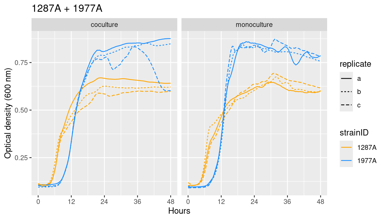
Figure 7: Growth curves (OD600 over 48 hours) of two strains in a competing pair (denoted by color and plot title). Line type denotes growth under pairwise competition (dashed line) or in monoculture. Plot panels depict the streptomycin concentration (ug/ml) under which growth was measured. Each co-culture condition was replicated six times while monoculture conditions were replicated three times. Plot panel rows depict growth in different streptomycin concentrations (ug/ml). Strain naming convention: 1287 = Citrobacter koserii 1287, 1977 = Psuedomonas chlororaphis 1977, A = Ancestral/Streptomycin sensitive, E = Evolved/Streptomycin resistant.
Source Code
---title: "Analyzing growth in pairs and monoculture"author: "Shane Hogle"date: todaylink-citations: trueabstract: "In the prior step we imported, smoothed, and calculated summary statistics for the species growth on the coculture plates. Here we will do some simple plots and analysis of the cocultures growth."---```{r}#| output: false#| warning: false#| error: false##### Librarieslibrary(tidyverse)library(here)library(fs)library(scales)source(here::here("R", "utils_gcurves.R"))##### Global variablesdata_raw <- here::here("_data_raw", "coculture_plate")data <- here::here("data", "coculture_plate")# make processed data directory if it doesn't existfs::dir_create(data)```# Read data```{r}#| output: false#| warning: false#| error: false##### growth summary datagcurves <- readr::read_tsv(here::here(data, "coculture_gcurves_smooth.tsv"))```# Plot growth curves## Difusion testPlot the co-cultures growing on M9 compared to the control (column 1 and 3)::: {#fig-01}```{r}#| fig-width: 9#| fig-height: 6gcurves %>%filter(str_detect(culture_type, "diffusion")) %>%filter(str_detect(strain, "NANA", negate=TRUE)) %>%ggplot() + ggplot2::geom_line(aes(x = hours, y = OD600_rollmean, lty = replicate, color = culture_type, group =interaction(well, plate_name))) + ggplot2::labs(x ="Hours", y ="OD600") + ggplot2::scale_x_continuous(breaks =seq(0, 48, 12), labels =seq(0, 48, 12)) +labs(y ="Optical density (600 nm)", x ="Hours", title ="Diffusion test") +facet_grid(evolution~strain)```Growth curves (OD600 over 48 hours) in monoculture for three replicates (line type) of each species (plot panel columns) and evolution status (plot panel rows). Line color indicates experimental conditions: Blue = "Double Media" which is standard inoculation into R2A growth medium with an adjacent well also containing R2A growth medium but with no inoculum. Green = diffusion test where bacteria are inoculated into M9 salts adjacent to a well containing R2A growth medium but with no inoculum. Red = diffusion test where bacteria are inoculated into R2A medium adjacent to a well containing M9 salts but with no inoculum. On the plate, column $n=\{1\dots11\}$ is connected to column $n+1$ with a 0.22 um membrane allowing free diffusion of resources and metabolic byproducts but not cells. These experiments were all conducted with no Streptomycin. Strain naming convention: 1287 = Citrobacter koserii 1287, 1977 = Psuedomonas chlororaphis 1977, A = Ancestral/Streptomycin sensitive, E = Evolved/Streptomycin resistant. :::## Monocultures and cocultures```{r}### Formatting and plotting functions# This function collects all the data from monocultures and cocultures for the selected species pair# only monoculture data from streptomycin concentrations tested in co-cultures is includedcollect_sp_pairs <-function(df, competition_pair, strep_thresh){ strainpairs <- stringr::str_split(competition_pair, "_")[[1]] df %>%mutate(streptomycin =if_else(plate_name =="plate01", 0, streptomycin)) %>%mutate(strainID =paste0(stringr::str_to_upper(stringr::str_sub(evolution, start =1, end=1)), str_extract(strain, "\\d+"))) %>%filter(strainID %in% strainpairs) %>%filter(str_detect(culture_type, "diffusion", negate = T)) %>%filter(streptomycin <= {{ strep_thresh }}) %>%filter((culture_type =="coculture"& competition_pair == {{ competition_pair}} ) | culture_type =="monoculture") %>%mutate(culture_type =factor(culture_type, levels =c("monoculture", "coculture"))) }# this function plots the output from the collect_sp_pairs functionplot_sp_pairs <-function(df, title, ncol){ straincols <-c("A1287"="orange", "E1287"="purple", "A1977"="dodgerblue", "E1977"="limegreen") ggplot2::ggplot(df) + ggplot2::geom_line(aes(x = hours, y = OD600_rollmean, color = strainID, lty = culture_type, group =interaction(well, plate_name))) + ggplot2::labs(x ="Hours", y ="OD600") + ggplot2::scale_x_continuous(breaks =seq(0, 48, 12), labels =seq(0, 48, 12)) + ggplot2::labs(y ="Optical density (600 nm), log scale", x ="Hours", title = {{title}}) + ggplot2::scale_color_manual(values = straincols) + ggplot2::scale_y_continuous(trans ="log", breaks =c(0, 0.25, 0.5, 1)) + ggplot2::facet_wrap(~streptomycin, ncol = {{ncol}}) + ggplot2::theme_bw()}```### Sensitive 1287 (A1287) + Resistant 1287 (E1287)"**Important!** we do not yet have monoculture data for A1287 at 64 and 256 ug/ml streptomycin!::: {#fig-02}```{r}#| fig-width: 9#| fig-height: 5collect_sp_pairs(gcurves, competition_pair ="A1287_E1287", strep_thresh =256) %>%plot_sp_pairs(title ="Sensitive 1287 (A1287) + Resistant 1287 (E1287)", ncol =4)```Growth curves (OD600 over 48 hours) of two strains in a competing pair (denoted by color and plot title). Line type denotes growth under pairwise competition (dashed line) or in monoculture. Plot panels depict the streptomycin concentration (ug/ml) under which growth was measured. Each co-culture condition was replicated six times while monoculture conditions were replicated three times. Plot panel rows depict growth in different streptomycin concentrations (ug/ml). Strain naming convention: 1287 = Citrobacter koserii 1287, 1977 = Psuedomonas chlororaphis 1977, A = Ancestral/Streptomycin sensitive, E = Evolved/Streptomycin resistant. :::### Sensitive 1977 (A1977) + Resistant 1977 (E1977)**Important!** A1977 monoculture results at 8 ug/ml streptomycin are strange, and I do not trust they are valid. The lag phase is much longer than at 12 or 16 ug/ml. I suspect this is from an experimental error and these curves should not be used. We can work to redo the measurements at 8 ug/ml::: {#fig-03}```{r}#| fig-width: 8#| fig-height: 5collect_sp_pairs(gcurves, competition_pair ="A1977_E1977", strep_thresh =24) %>%plot_sp_pairs(title ="Sensitive 1977 (A1977) + Resistant 1977 (E1977)", ncol =3)```Growth curves (OD600 over 48 hours) of two strains in a competing pair (denoted by color and plot title). Line type denotes growth under pairwise competition (dashed line) or in monoculture. Plot panels depict the streptomycin concentration (ug/ml) under which growth was measured. Each co-culture condition was replicated six times while monoculture conditions were replicated three times. Plot panel rows depict growth in different streptomycin concentrations (ug/ml). Strain naming convention: 1287 = Citrobacter koserii 1287, 1977 = Psuedomonas chlororaphis 1977, A = Ancestral/Streptomycin sensitive, E = Evolved/Streptomycin resistant. :::### Sensitive 1287 (A1287) + Sensitive 1977 (A1977)**Important!** A1977 monoculture results at 8 ug/ml streptomycin are strange, and I do not trust they are valid. The lag phase is much longer than at 12 or 16 ug/ml. I suspect this is from an experimental error and these curves should not be used. We can work to redo the measurements at 8 ug/ml::: {#fig-04}```{r}#| fig-width: 9#| fig-height: 6collect_sp_pairs(gcurves, competition_pair ="A1287_A1977", strep_thresh =24) %>%plot_sp_pairs(title ="Sensitive 1287 (A1287) + Sensitive 1977 (A1977)", ncol =3)```Growth curves (OD600 over 48 hours) of two strains in a competing pair (denoted by color and plot title). Line type denotes growth under pairwise competition (dashed line) or in monoculture. Plot panels depict the streptomycin concentration (ug/ml) under which growth was measured. Each co-culture condition was replicated six times while monoculture conditions were replicated three times. Plot panel rows depict growth in different streptomycin concentrations (ug/ml). Strain naming convention: 1287 = Citrobacter koserii 1287, 1977 = Psuedomonas chlororaphis 1977, A = Ancestral/Streptomycin sensitive, E = Evolved/Streptomycin resistant.:::### Resistant 1287 (E1287) + Sensitive 1977 (A1977)**Important!** A1977 monoculture results at 8 ug/ml streptomycin are strange, and I do not trust they are valid. The lag phase is much longer than at 12 or 16 ug/ml. I suspect this is from an experimental error and these curves should not be used. We can work to redo the measurements at 8 ug/ml::: {#fig-05}```{r}#| fig-width: 9#| fig-height: 6collect_sp_pairs(gcurves, competition_pair ="E1287_A1977", strep_thresh =24) %>%plot_sp_pairs(title ="Resistant 1287 (E1287) + Sensitive 1977 (A1977)", ncol =3)```Growth curves (OD600 over 48 hours) of two strains in a competing pair (denoted by color and plot title). Line type denotes growth under pairwise competition (dashed line) or in monoculture. Plot panels depict the streptomycin concentration (ug/ml) under which growth was measured. Each co-culture condition was replicated six times while monoculture conditions were replicated three times. Plot panel rows depict growth in different streptomycin concentrations (ug/ml). Strain naming convention: 1287 = Citrobacter koserii 1287, 1977 = Psuedomonas chlororaphis 1977, A = Ancestral/Streptomycin sensitive, E = Evolved/Streptomycin resistant.:::### Sensitive 1287 (A1287) + Resistant 1977 (E1977)**Important!** we do not yet have monoculture data for A1287 at 64 and 256 ug/ml streptomycin!::: {#fig-06}```{r}#| fig-width: 9#| fig-height: 6collect_sp_pairs(gcurves, competition_pair ="A1287_E1977", strep_thresh =256) %>%plot_sp_pairs(title ="Sensitive 1287 (A1287) + Resistant 1977 (E1977)", ncol =4)```Growth curves (OD600 over 48 hours) of two strains in a competing pair (denoted by color and plot title). Line type denotes growth under pairwise competition (dashed line) or in monoculture. Plot panels depict the streptomycin concentration (ug/ml) under which growth was measured. Each co-culture condition was replicated six times while monoculture conditions were replicated three times. Plot panel rows depict growth in different streptomycin concentrations (ug/ml). Strain naming convention: 1287 = Citrobacter koserii 1287, 1977 = Pseudomonas chlororaphis 1977, A = Ancestral/Streptomycin sensitive, E = Evolved/Streptomycin resistant.:::### Sensitive 1287 (A1287) + Resistant 1977 (E1977)**Important!** E1977 monoculture replicate at 4096 ug/ml should be excluded - growth curve is messed up::: {#fig-07}```{r}#| fig-width: 10#| fig-height: 6collect_sp_pairs(gcurves, competition_pair ="E1287_E1977", strep_thresh =4096) %>%plot_sp_pairs(title ="Resistant 1287 (E1287) + Resistant 1977 (E1977)", ncol =5)```Growth curves (OD600 over 48 hours) of two strains in a competing pair (denoted by color and plot title). Line type denotes growth under pairwise competition (dashed line) or in monoculture. Plot panels depict the streptomycin concentration (ug/ml) under which growth was measured. Each co-culture condition was replicated six times while monoculture conditions were replicated three times. Plot panel rows depict growth in different streptomycin concentrations (ug/ml). Strain naming convention: 1287 = Citrobacter koserii 1287, 1977 = Psuedomonas chlororaphis 1977, A = Ancestral/Streptomycin sensitive, E = Evolved/Streptomycin resistant.:::