Analysis of quartet competition

Abstract

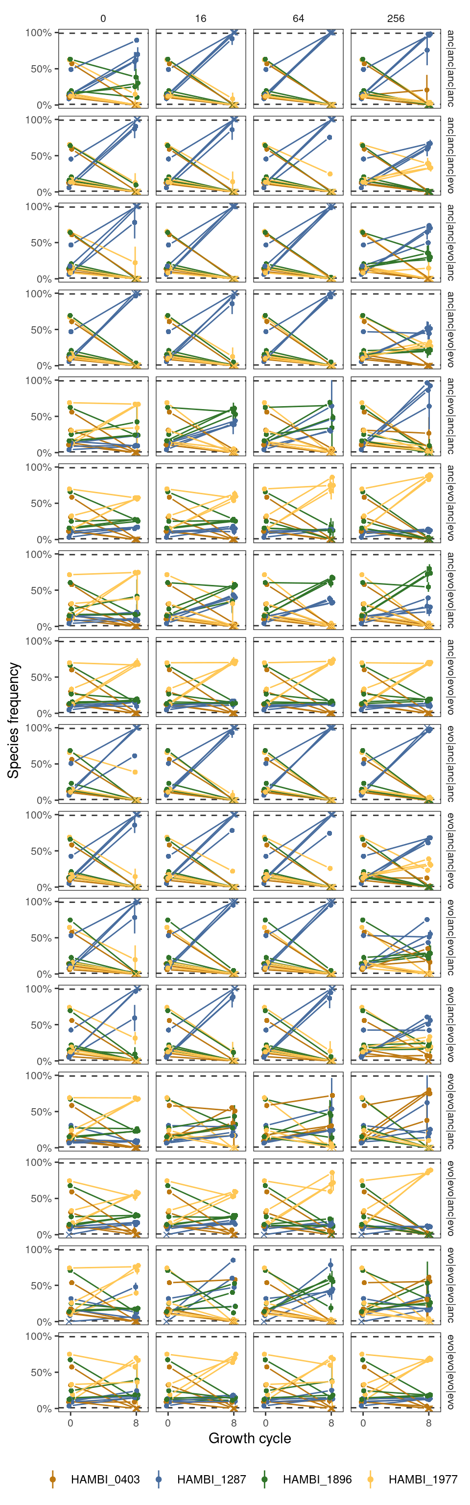
Here we analyze the community outpcomes from all competing species quartets.

1 Setup

1.1 Libraries

library(tidyverse)
library(here)
library(fs)
library(scales)
library(patchwork)
library(broom)
library(ggraph)
library(ggh4x)
library(tidygraph)
source(here::here("R", "utils_generic.R"))

1.2 Global variables

data <- here::here("data", "communities")
# make processed data directory if it doesn't exist
fs::dir_create(data)

2 Read data

2.1 Species abundances

samp_quarts <- readr::read_tsv(here::here(data, "4sps_compiled.tsv")) %>% 
  dplyr::rename(f = f_thresh)

3 Format

Create a metadata tibble that contains faceting information

md <- samp_quarts %>% 
  dplyr::select(sample, strainID, evo_hist, target_f_masterplate) %>% 
  # make a combined evolution and species identifier and extract the community ID
  dplyr::mutate(strainID = paste0("H", str_extract(strainID, "\\d+"))) %>% 
  dplyr::group_by(sample) %>% 
  dplyr::mutate(n = 1:n()) %>% 
  ungroup() %>% 
  tidyr::pivot_wider(id_cols = c(sample), values_from = c(strainID, evo_hist, target_f_masterplate), names_from = n) %>% 
  mutate(sps = paste(strainID_1, strainID_2, strainID_3, strainID_4, sep = "-"),
         f0 = paste(target_f_masterplate_1, target_f_masterplate_2, target_f_masterplate_3, target_f_masterplate_4, sep = "-"),
         hist = paste(evo_hist_1, evo_hist_2, evo_hist_3, evo_hist_4, sep = "|")) %>% 
  dplyr::select(sample, sps, f0, hist)

Combine into a final tibble

t0 <- samp_quarts %>% 
  dplyr::filter(community_type == "masterplate") %>% 
  dplyr::select(-strep_conc, -replicate) %>% 
  full_join(tibble(transfers = c(0, 0, 0, 0), strep_conc = c(0, 16, 64, 256)),
            by = join_by(transfers),
            relationship = "many-to-many")

t8 <- samp_quarts %>% 
  dplyr::filter(community_type == "experiment")

tf <- bind_rows(t0, t8) %>% 
  left_join(md, by = join_by(sample)) %>% 
  dplyr::summarize(ggplot2::mean_cl_boot(f),
                    .by = c("sps", "f0", "hist", "strep_conc", "transfers", "strainID")) %>% 
  mutate(ymin = if_else(is.na(ymin), y, ymin),
         ymax = if_else(is.na(ymax), y, ymax)) %>% 
  mutate(extinct = if_else(y <= 0.01 | y >= 0.99, "extinct", "coexist"))

4 Plot

spcols <- c("HAMBI_0403" = "#bd7811", "HAMBI_1287" = "#476c9e", "HAMBI_1896" = "#31752a", "HAMBI_1977" = "#ffc755")

pj <- ggplot2::position_jitterdodge(jitter.width=0.0,
                           jitter.height = 0.0,
                           dodge.width = 0.5,
                           seed=9)

p4sps <- ggplot(tf, aes(x = transfers, y = y, group = interaction(strainID, f0, strep_conc, hist))) +
  geom_hline(yintercept=0.01, color = "grey20", lty = 2) +
  geom_hline(yintercept=0.99, color = "grey20", lty = 2) +
  ggplot2::geom_linerange(aes(ymin = ymin, ymax = ymax, color = strainID), position = pj) + 
  ggh4x::geom_pointpath(aes(color = strainID, shape = extinct), position = pj, mult = 0.2) +
  facet_grid(hist ~ strep_conc) +
  ggplot2::labs(x = "Growth cycle", y = "Species frequency", color = "Species") +
  ggplot2::scale_y_continuous(limits = c(0, 1), breaks = c(0, 0.5, 1), labels = percent) + #trans = "sqrt",
  ggplot2::scale_x_continuous(limits = c(-1, 9), breaks = c(0, 8)) +
  scale_shape_manual(values = c(16, 4), guide = "none") +
  scale_color_manual(values = spcols) +
  ggplot2::theme_bw() + 
  ggplot2::theme(strip.background = element_blank(),
        legend.position = "bottom", 
        panel.grid = element_blank(),
        legend.title = element_blank(),
        axis.text = element_text(size = 8),
        strip.text = element_text(size = 8))

Figure 1: Compositions of all species together at 4 different streptomycin concentrations (0, 16, 64, and 256 μg/ml; grid columns) and the 16 evolutionary history combinations tested (grid rows). The evolutionary histories are always in the same species order (HAMBI_0403, HAMBI_1287, HAMBI_1896, HAMBI_1977). In each evolutionary history and streptomycin treatment combination there are four different starting fractions where each species is allowed to start from high abundance once and from rare three times Points depict species relative abundance (vertical axis) at the start of the experiment and after eight 48-hour growth cycles (horizontal axis). Point crosses represent whether the species is below/above a 1%/99% threshold where it is effectively extinct/excluded all other competitors. Points are the mean over at least 2 replicates and line ranges represent confidence limits of the population mean from a basic nonparametric bootstrap.