Designing two-species subcommunities
Abstract
This notebook creates and lays out the steps for constructing the experimental species pairs for this experiment. It is inspired by the method outlined in this paper: Full factorial construction of synthetic microbial communities, eLife 13:RP101906. Note that we did not include competition between the evolved and ancestral form of each species because they would not be distinguishable using 16S rRNA amplicon sequencing. However, they could concievably be competed through CFU counting on a counter selective agar containing streptomycin.
1 Setup
1.1 Libraries
1.2 Global variables
1.3 Functions and vars
Species color vector
Show/hide code
my_colors <- c(
  "ANC_0403_10" = "#ffaaaa", "ANC_0403_70" = "#aa0000", "ANC_0403_80" = "#aa0000", "ANC_0403_90" = "#aa0000",
  "ANC_1287_10" = "#ffeeaa", "ANC_1287_70" = "#d4aa00", "ANC_1287_80" = "#d4aa00", "ANC_1287_90" = "#d4aa00",
  "ANC_1896_10" = "#ccffaa", "ANC_1896_70" = "#44aa00", "ANC_1896_80" = "#44aa00", "ANC_1896_90" = "#44aa00",
  "ANC_1977_10" = "#aaccff", "ANC_1977_70" = "#0055d4", "ANC_1977_80" = "#0055d4", "ANC_1977_90" = "#0055d4",
  "EVO_0403_10" = "#ffaaee", "EVO_0403_70" = "#ff00cc", "EVO_0403_80" = "#ff00cc", "EVO_0403_90" = "#ff00cc",
  "EVO_1287_10" = "#ffccaa", "EVO_1287_70" = "#ff6600", "EVO_1287_80" = "#ff6600", "EVO_1287_90" = "#ff6600",
  "EVO_1896_10" = "#aaffee", "EVO_1896_70" = "#00ffcc", "EVO_1896_80" = "#00ffcc", "EVO_1896_90" = "#00ffcc",
  "EVO_1977_10" = "#ccaaff", "EVO_1977_70" = "#7f2aff", "EVO_1977_80" = "#7f2aff", "EVO_1977_90" = "#7f2aff"
  )
For plotting plates
2 Construct pair combinations
Get all possible pairs while excluding combinations of ANC/EVO of the same species
Make plate layouts for the 2-species combos
Show/hide code
combos02_filt_well_left <- combos02_filt %>%
  mutate(a = paste(a, 90, sep = "_"),
         b = paste(b, 10, sep = "_")) %>%
  add_count(a, name = "a_count") %>%
  add_count(b, name = "b_count") %>%
  arrange(desc(a_count), a) %>%
  mutate(row = rep(LETTERS[1:n_distinct(a)],
                   times = rep(c(n_distinct(a):2)[n_distinct(a):2%%2 == 0], each = 2))) %>%
  group_by(row) %>%
  arrange(desc(b_count), b) %>%
  mutate(col = str_pad(1:length(row), 2, pad = "0")) %>%
  ungroup() %>%
  mutate(well = paste0(row, col))

combos02_filt_well_right <- combos02_filt %>%
  mutate(a = paste(a, 10, sep = "_"),
         b = paste(b, 90, sep = "_")) %>%
  add_count(a, name = "a_count") %>%
  add_count(b, name = "b_count") %>%
  arrange(desc(a_count), a) %>%
  mutate(row = rep(LETTERS[1:n_distinct(a)],
                   times = rep(c(n_distinct(a):2)[n_distinct(a):2%%2 == 0], each = 2))) %>%
  group_by(row) %>%
  arrange(desc(b_count), b) %>%
  mutate(col = str_pad(1:length(row)+6, 2, pad = "0")) %>%
  ungroup() %>%
  mutate(well = paste0(row, col)) %>%
  rename(a = b, b = a )

combos02_filt_well <- bind_rows(combos02_filt_well_left, combos02_filt_well_right)
2.1 Format and save
Show/hide code
combos02_filt_well %>%
  group_by(a, b) %>%
  mutate(microcosm_id = cur_group_id()) %>%
  ungroup() %>%
  mutate(a_sp = paste0(str_split_i(a, "_", 2), stringr::str_extract(str_split_i(a, "_", 1), "^.{1}")),
         b_sp = paste0(str_split_i(b, "_", 2), stringr::str_extract(str_split_i(b, "_", 1), "^.{1}")),
         a_f = str_split_i(a, "_", 3),
         b_f = str_split_i(b, "_", 3)) %>%
  arrange(well) %>%
  dplyr::select(microcosm_id, well, a, a_sp, a_f, b, b_sp, b_f) %>%
  readr::write_tsv(here::here(data, "pairs_sample_composition_wide.tsv"))
Show/hide code
combos02_filt_well %>%
  group_by(a, b) %>%
  mutate(microcosm_id = cur_group_id()) %>%
  ungroup() %>%
  dplyr::select(a:b, well, microcosm_id) %>%
  tidyr::pivot_longer(c(-well, -microcosm_id)) %>%
  tidyr::separate(value, c("evo_hist", "strainID", "target_f")) %>%
  dplyr::mutate(evo_hist = stringr::str_to_lower(evo_hist),
                strainID = paste0("HAMBI_", strainID),
                target_f = as.numeric(target_f)/100,
                n_species = 2) %>%
  dplyr::select(-name) %>%
  dplyr::relocate(microcosm_id, n_species) %>%
  readr::write_tsv(here::here(data, "pairs_sample_composition_long.tsv"))
3 Pipetting
Proceed in the order of steps below to construct master plates used to inoculate different conditions
3.1 First pipetting step
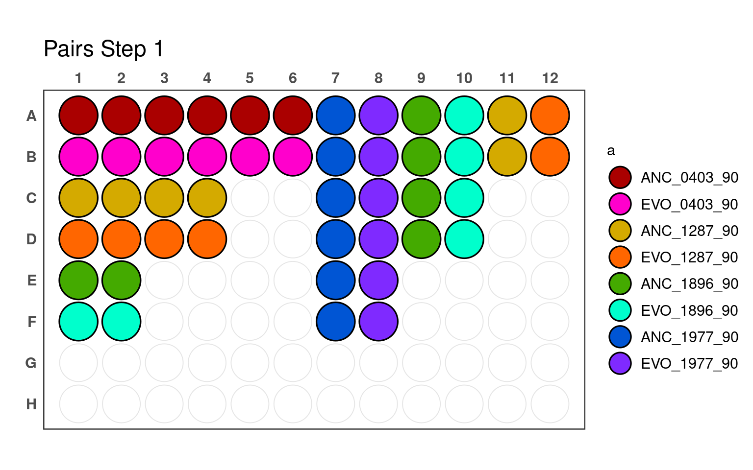
_90) or 10% (e.g., _10).
3.2 Second pipetting step

_90) or 10% (e.g., _10).