Formatting Rbec output from 2025-05-02 sequenced by BTK Turku using custom HAMBI Illumina v3 primers

Abstract

Results are from samples containing the mixture of 8 strains (both anc/evo form for each species) as well as one single triplet, and all the pairs with 50:50 abundance.

1 Setup

1.1 Libraries

library(tidyverse)
library(here)
library(fs)
library(archive)
library(scales)
source(here::here("R", "utils_generic.R"))
source(here::here("R", "communities", "amplicon", "utils_amplicon.R"))

1.2 Global variables

data_raw <- here::here("_data_raw", "communities", "20250502_BTK_illumina_v3")
data <- here::here("data", "communities", "20250502_BTK_illumina_v3")
amplicontar <- here::here(data_raw, "rbec_output.tar.gz")

# make processed data directory if it doesn't exist
fs::dir_create(data)

# create temporary location to decompress
tmpdir <- fs::file_temp()

2 Read metadata

mddf <- readr::read_tsv(here::here(data_raw, "20250502_BTK_illumina_v3_metadata.tsv")) %>% 
  mutate(sample = str_trim(sample))
spdf <- readr::read_tsv(here::here(data_raw, "sample_compositions.tsv")) %>% 
  mutate(sample = str_trim(sample))

3 Read Rbec raw counts tables

3.1 Untar Rbec output tarball

archive::archive_extract(
  amplicontar,
  dir = tmpdir,
  files = NULL,
  options = character(),
  strip_components = 0L
)

3.2 Setup directory structure

tabdir <- here::here(tmpdir, "rbec_output")
samppaths <- fs::dir_ls(tabdir)
sampnames <- path_split(samppaths) %>% 
  map_chr(dplyr::last)

3.3 Read

straintabs <- paste0(samppaths, "/strain_table.txt") %>% 
  set_names(sampnames) %>% 
  map_df(
  read_tsv,
  skip = 1,
  col_names = c("rRNA16S_locus","count"),
  show_col_types = FALSE, 
  .id = "sample")

3.4 Clean up

# remove decompressed directory from temp location
fs::dir_delete(tmpdir)

4 Format

straintabs_norm <- straintabs %>% 
  # Calls function that normalize counts by 16S copy number
  normalize_by_copy() %>% 
  # Calls function that completes all combinations of 23 species
  # this is important because some species go extinct that should be in the samples
  # and we need to have those in the final table
  complete_combos() %>% 
  # removes any extra whitespace on sample names
  mutate(sample = str_trim(sample))

Make final table

# Later we will take advantage of the fact that for species not supposed to be
# in a sample the prior left_join will have filled the evo_hist category with an
# NA. We can then filter using this NA value
finaltable <- left_join(straintabs_norm, mddf, by = join_by(sample)) %>% 
  left_join(spdf, by = join_by(sample, strainID)) %>% 
  group_by(sample) %>% 
  dplyr::select(-genus, -species) %>% 
  mutate(f_raw = count_correct/sum(count_correct),
         sample_tot_raw = sum(count_correct)) %>% 
  ungroup() %>% 
  relocate(sample_tot_raw, f_raw, target_f, evo_hist, .after = count_correct)

5 Analysis

Let’s quickly compare and look the at number of reads from the different kinds of experiment categories. Negative controls are samples from the experiment that contained growth medium but no cells. We included them to make sure that there was not contamination between wells during the experiment. Positive controls contain a mixsture of all 23 species (not sure why this was done), and some wells are just empty but were processed/sequenced anyway for convenience of the person preparing the libraries. Experiment samples are those that came from the actual experiment, and masterplate samples are the defined mixtures we made to inoculate the experiment. We sequenced these masterplates so that we would have T0 information for each experimental treatment.

finaltable %>% 
  dplyr::select(sample, sample_tot_raw, community_type) %>% 
  distinct() %>% 
  ggplot(aes(x = sample_tot_raw)) +
  geom_histogram(bins = 20, aes(fill = community_type)) +
  scale_x_log10() + 
  annotation_logticks(sides = "b", color="grey30") +
  labs(y = "Sample count", x = "Total reads per sample")  +
  facet_wrap(~ community_type, scales="free_y", nrow = 2)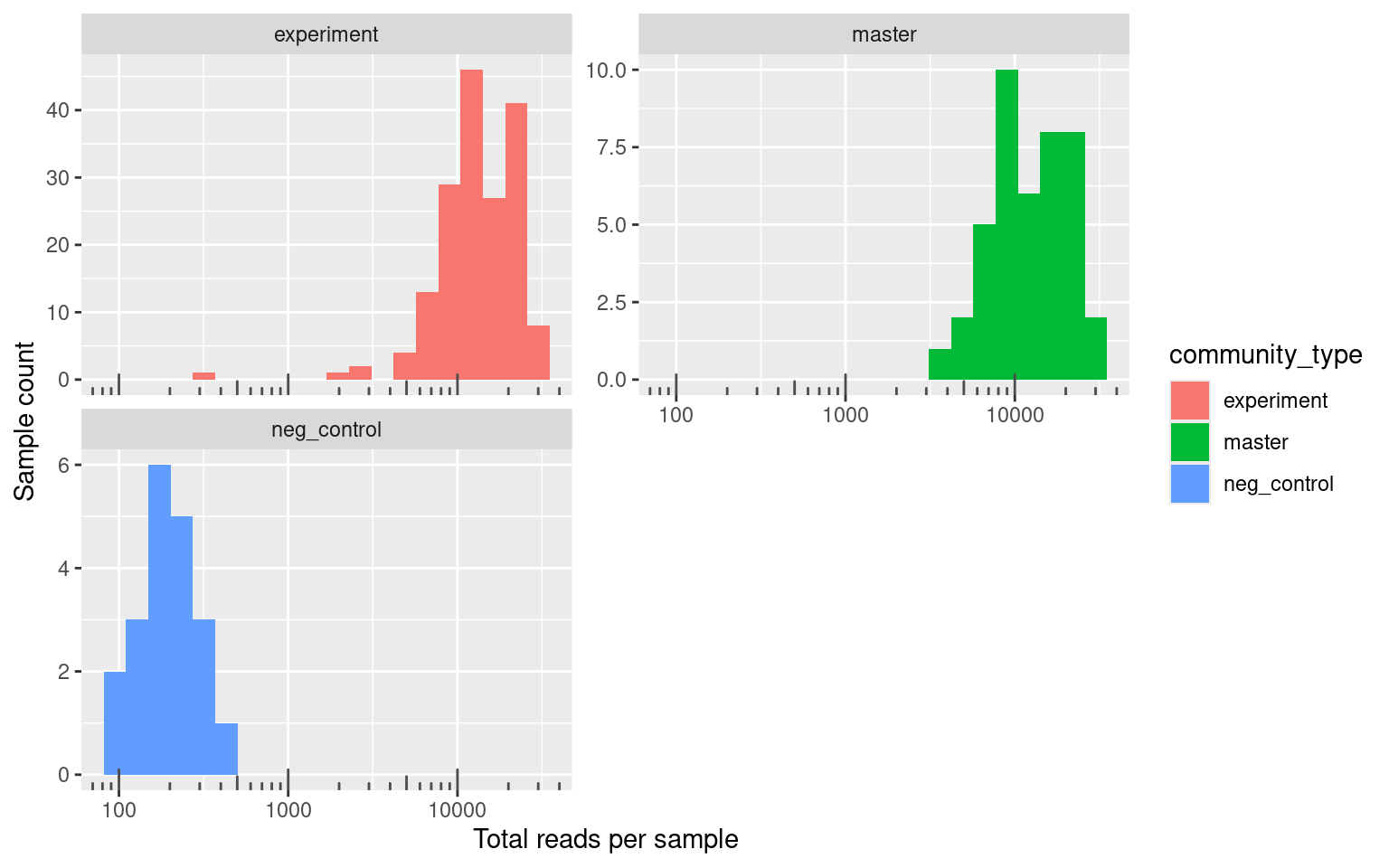

Figure 1: Frequency distribution of total read counts per sample in the experimental samples (red) and the negative controls (blue).

The smallest number of reads in the experimental samples is 340 and the mean is 1.5133^{4} which is considerably more than the smallest number of reads 99 and the mean 199.6 in the negative controls.

Overall this looks pretty good. From the figure above we can see that there is a clear disjoint between about 1000 reads that separate samples that are negative controls and the experimental samples. There is one experimental sample with fewer than 1000 reads. It is likely that this sample failed or it is from a condition where no species survived.

5.1 Negative controls

Read optical density data for the experiment

OD <- readr::read_tsv(here::here("_data_raw", "communities", "optical_density", "20250425_8sp_5050pairs", "optical_density_formatted.tsv")) %>% 
  mutate(sample2 = case_when(str_detect(sample, "com_") ~ paste0("8", str_extract(sample, "_\\d+$")),
                             str_detect(sample, "^3_p") ~ paste0("3_c01_", str_extract(well, "[:upper:]"), str_pad(str_extract(well, "\\d+"), 2, "left", pad = "0")),
                             str_detect(sample, "^p\\d+") ~ paste0("2_", str_extract(sample, "\\d+"), "_", str_extract(well, "[:upper:]"), str_pad(str_extract(well, "\\d+"), 2, "left", pad = "0")),
                             str_detect(sample, "^p") ~ str_to_upper(sample)))

Rows: 960 Columns: 7
── Column specification ────────────────────────────────────────────────────────
Delimiter: "\t"
chr (2): sample, well
dbl (5): transfers, n_species, strep_conc, replicate, OD

ℹ Use `spec()` to retrieve the full column specification for this data.
ℹ Specify the column types or set `show_col_types = FALSE` to quiet this message.

First just checking the negative controls

OD %>% 
  filter(str_detect(sample, "neg_control")) %>% 
  ggplot(aes(x = OD)) +
  geom_histogram(bins = 10) +
  geom_vline(xintercept = 0.1, color = "red") + 
  labs(y = "Sample count", x = "Sample optical density")  +
  facet_grid(~ transfers, scales="free_y")

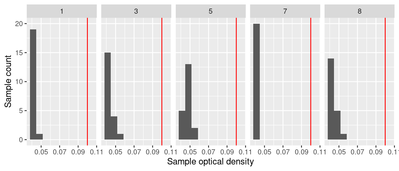
Negative controls look good. OD in all negative controls is low (<0.07)

5.2 Positive controls

No positive controls included in this run

5.3 Misassigned reads

These libraries were only prepared with samples containing HAMBI_0403, HAMBI_1287, HAMBI_1896, and HAMBI_1977 so any time species other than these show up is just an incorrect assignment by Rbec or index leakage/crosstalk from the positive community controls. Let’s check quickly how many of these there are…

finaltable %>% 
  filter(!str_detect(strainID, "0403|1287|1896|1977")) %>% 
  filter(count_correct > 0) %>% 
  arrange(desc(count_correct))

There are only a couple of random reads per experimental sample so we can safely ignore them. Since there was no positive control included here the off-target species must come from missassignments and not index leakage from community control.

5.4 Samples with few total reads

Some of the experimental pairs had streptomycin concentrations higher than any of the species individually could tolerate. We would expect then that no species would grow successfully in these samples and that the overall biomass would be very low, thus resulting in a low number of recovered reads from these samples.

To look into this. first let’s check which samples have very low OD600 in the endpoint samples. We’ll filter out samples with an OD of less than 0.1 or samples with fewer than 3000 reads. It is generally good practice to exclude samples with low number of reads.

left_join(finaltable, OD, 
                 by = join_by(sample == sample2)) %>% 
  filter(transfers.y == 8) %>% 
  filter(OD < 0.1 | sample_tot_raw < 1000) %>% 
  distinct(sample, community_type, OD, sample_tot_raw) %>%
  arrange(sample_tot_raw)

Warning in left_join(finaltable, OD, by = join_by(sample == sample2)): Detected an unexpected many-to-many relationship between `x` and `y`.
ℹ Row 24 of `x` matches multiple rows in `y`.
ℹ Row 97 of `y` matches multiple rows in `x`.
ℹ If a many-to-many relationship is expected, set `relationship =
  "many-to-many"` to silence this warning.

df <- left_join(finaltable, OD, 
                 by = join_by(sample == sample2)) %>% 
  filter(transfers.y == 8) %>% 
  filter(OD < 0.1 | sample_tot_raw < 1000) %>% 
  distinct(sample, community_type, OD, sample_tot_raw) 

Warning in left_join(finaltable, OD, by = join_by(sample == sample2)): Detected an unexpected many-to-many relationship between `x` and `y`.
ℹ Row 24 of `x` matches multiple rows in `y`.
ℹ Row 97 of `y` matches multiple rows in `x`.
ℹ If a many-to-many relationship is expected, set `relationship =
  "many-to-many"` to silence this warning.

lowread_samps <- df %>% 
  filter(sample_tot_raw < 1000 & community_type == "experiment") %>% 
  distinct(sample) %>% 
  pull(sample)

There is only one low-read sample. It corresponds to a pair with both ancestral HAMBI_1977 and HAMBI_0403 in 256 ug/ml streptomycin. From monoculture results we know this streptomycin concentration is outside the tolerable range for these two species. Indeed, the OD in this sample at time point 8 is 0.046, which indicates very low biomass at the experiment’s conclusion.

5.5 Filter to target species

Exclude positive and negative controls and also exclude species that are not in the focal 4

finaltable_exp_mstr <- finaltable %>% 
  filter(community_type %nin% c("empty", "neg_control", "pos_control")) %>% 
  filter(sample %nin% lowread_samps) %>% 
  filter(strainID %in% c("HAMBI_0403", "HAMBI_1287", "HAMBI_1896", "HAMBI_1977")) %>% 
  group_by(sample) %>% 
  mutate(f_raw_targetsp = count_correct/sum(count_correct),
         sample_tot_targetsp = sum(count_correct)) %>% 
  ungroup() %>% 
  relocate(c(sample_tot_targetsp, f_raw_targetsp), .after = f_raw)

5.6 Master plates samples

Crosstalk on master plates is quite good - usually < 1% frequency.

finaltable_exp_mstr %>% 
  filter(str_detect(community_type, "master")) %>%
  filter(is.na(evo_hist)) %>% 
  filter(f_raw_targetsp > 0.01 ) %>% 
  dplyr::select(sample, strainID, f_raw_targetsp) %>% 
  arrange(desc(f_raw_targetsp))

finaltable_exp_mstr %>% 
  filter(str_detect(community_type, "master")) %>% 
  filter(is.na(evo_hist)) %>% 
  contam_histogram(trans=TRUE, x = f_raw_targetsp) +
  labs(x = "Species frequency", y = "Sample count") +
  ggtitle("Frequency distribution of each species in master plate samples where it should not be")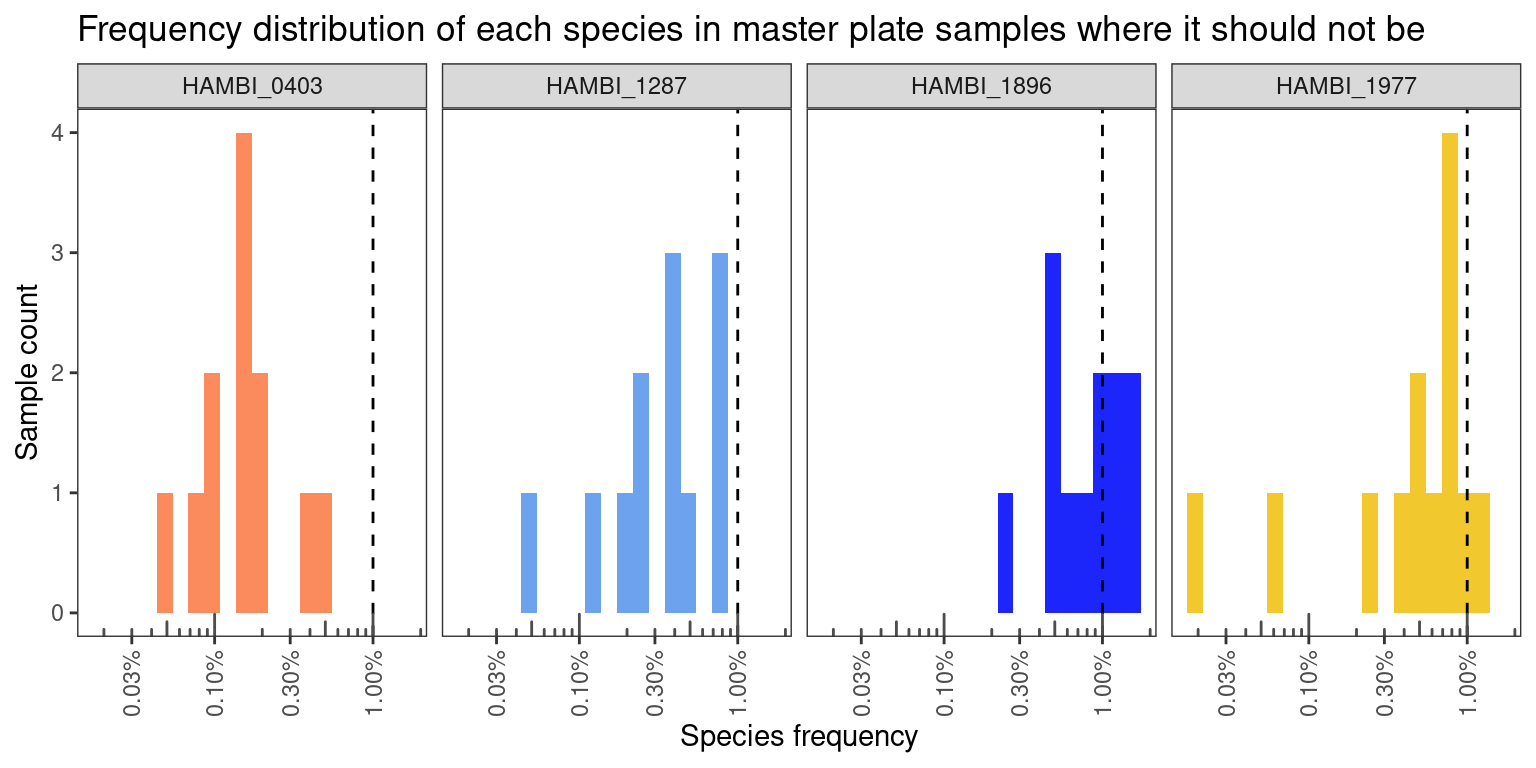

Figure 2: Frequency distribution of each species in masterplate samples where it should not occur and where it exceeds a 3% threshold.

5.7 Experimental samples

finaltable_exp_mstr %>% 
  filter(!str_detect(community_type, "master")) %>%
  filter(is.na(evo_hist)) %>% 
  filter(f_raw_targetsp > 0.01 ) %>% 
  dplyr::select(sample, strainID, f_raw_targetsp) %>% 
  arrange(desc(f_raw_targetsp))

There are 39 samples (18% of 213 samples) that exceed a 1% crosstalk threshold. 28 samples (13% of 213 samples) have contamination <= 3% and 12 samples (6 % of 213 samples) have > 3% of a species that should not be there. In most cases the species in highly contaminated samples is HAMBI_1896. In general, this level of contamination is quite low and samples with contamination greater than 3% are just crosstalk outliers.

finaltable_exp_mstr %>% 
  filter(str_detect(community_type, "experiment")) %>% 
  contaminated_barplot(threshold=0.01, quartet = FALSE, y=f_raw_targetsp) +
  ggtitle("Experiment samples with > 1% contamination")

Figure 3: Species composition of experiment samples that contain > 3% of a species that shouldn’t be there (shown in grey to black).

contamtrios <- finaltable_exp_mstr %>% 
  filter(n_species == 3) %>% 
  filter(is.na(evo_hist)) %>% 
  filter(f_raw_targetsp > 0.13  ) %>% 
  pull(sample)

Only 6 trio samples look really bad (~50 % contamination). Again, I think we should only exclude samples where the contamination is very high (over ~50% of the sample) but those with around 10% or less contaminant I think can be retained, and I will discard the contaminating sequences. Interestingly the lower-level contamination (3% > contamination > 13%) seems to be mostly from from HAMBI_1896. The high level contamination is always in well C01 on 6 different plates ().

5.8 Plot

5.8.1 Pairs and trios

finaltable_exp_mstr %>% 
  filter(str_detect(community_type, "experiment")) %>% 
  filter(n_species != 8) %>% 
  group_by(sample) %>% 
  mutate(id = cur_group_id()) %>% 
  ungroup() %>% 
  mutate(facet = ntile(id, 5)) %>% 
  # to make sure ntile doesnt split up facets
  group_by(sample) %>% 
  mutate(facet = first(facet)) %>% 
  ungroup() %>% 
  contaminated_barplot(threshold = 0, quartet = TRUE, y=f_raw_targetsp) +
  ggtitle("All experimental pairs and trios") +
  facet_wrap(~facet, scales="free_x", nrow=5) +
  theme(
    strip.background = element_blank(),
    strip.text.x = element_blank(),
    legend.position = "bottom"
    )

Figure 4: Species composition of all experiment trio samples. Species that should not be present in a sample are shown in grey to black.

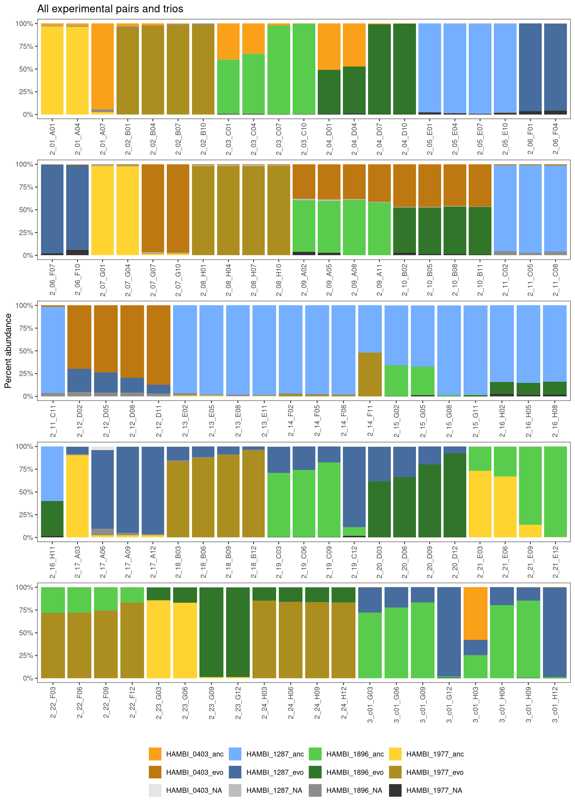
At a birds-eye view this looks pretty good overall.

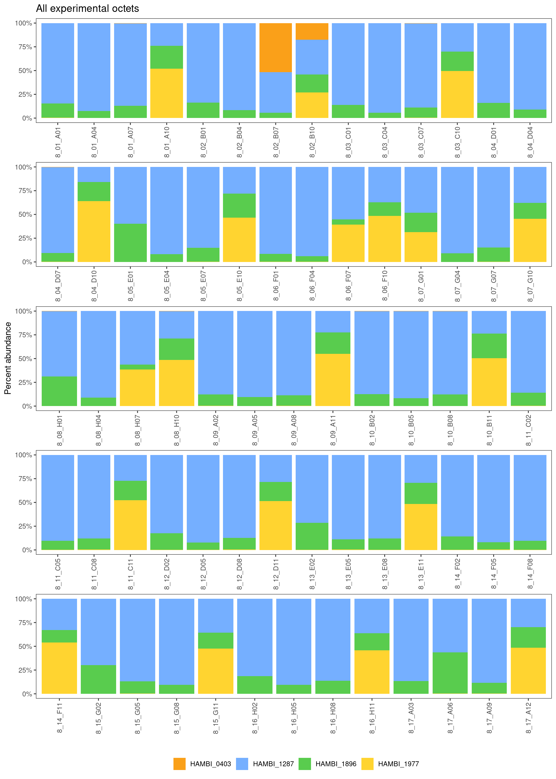
5.8.2 Octets

Again, one weakness of this approach is that there is no way to tell from this data whether an octets is contaminated because every octet (by definition) is inoculated with all of the 4 species at different frequencies and with different evolutionary histories. Thus we would expect to see either all 4 species present or a subset of the 4 species in the quartet samples, but we cannot tell if these patterns come from contamination or not. Moving forward we just have to assume that the quartets are OK… However, we’ve found so little contamination in our other experimental samples and all samples were handled in the experiment and processed for sequence library preparation in the same way. I think it is safe to assume that contamination in the quartets is minimal issue.

finaltable_exp_mstr %>% 
  filter(str_detect(community_type, "experiment")) %>% 
  filter(n_species == 8) %>% 
  dplyr::select(sample, strainID, count_correct) %>% 
  distinct() %>% 
  group_by(sample) %>% 
  mutate(f_raw_targetsp = count_correct/sum(count_correct)) %>% 
  mutate(id = cur_group_id()) %>% 
  ungroup() %>% 
  mutate(facet = ntile(id, 5)) %>% 
  # to make sure ntile doesnt split up facets
  group_by(sample) %>% 
  mutate(facet = first(facet)) %>% 
  ungroup() %>% 
  ggplot() +
    geom_col(aes(x = sample, y = f_raw_targetsp, fill = strainID)) +
    labs(y = "Percent abundance", x = "", fill = "") +
    scale_fill_manual(values = c("HAMBI_0403" = "#faa019",
              "HAMBI_1287" = "#75afff",
              "HAMBI_1896" = "#59cc4e",
              "HAMBI_1977" = "#ffd430")
              ) +
    scale_y_continuous(labels = percent) +
    scale_x_discrete(guide = guide_axis(angle=90)) +
    theme_bw() + 
    theme(panel.grid = element_blank(), legend.position = "right") +
    ggtitle("All experimental octets") +
    facet_wrap(~facet, scales="free_x", nrow=5) +
    theme(
    strip.background = element_blank(),
    strip.text.x = element_blank(),
    legend.position = "bottom"
    )

Figure 5: Species composition of all experiment 8 strain samples.

6 Export

finaltable_exp_mstr_export <- finaltable_exp_mstr %>% 
  # first remove samples with low read count (< 3000 reads)
  filter(sample %nin% lowread_samps) %>% 
  # exclude any remaining counts from species that shouldnt be there using again
  # the fact that evo_hist should be NA for these species
  filter(!is.na(evo_hist)) %>% 
  # because we set 3% as our limit of detection we set read counts of species
  # less than 3% to 0
  mutate(count_correct_thresh = if_else(f_raw_targetsp <= 0.03, 0, count_correct)) %>% 
  # now calculate a new relative abundance based only on the species that should
  # be present and that are > 3% relative abundance
  group_by(sample) %>% 
  mutate(f_thresh = count_correct_thresh/sum(count_correct_thresh)) %>% 
  ungroup() %>%
  # for marking which sequencing batch these came from 
  mutate(batch = "run20250502") %>% 
  dplyr::select(sample, strainID, evo_hist, count_correct_thresh, f_thresh,
                target_f_masterplate = target_f, replicate, strep_conc, 
                transfers, n_species, community_type, plate_well, batch)

6.1 Pairs

finaltable_exp_mstr_export %>%
  filter(n_species == 2) %>%
  arrange(sample) %>%
  # reformating to be compatible with other pair data
  mutate(sample = if_else(
    community_type == "master",
    paste0("P", 
           str_extract(sample, pattern = '(?<=2_)\\d{2}'), "_s_0"),
    paste0("P",
           str_extract(sample, pattern = '(?<=2_)\\d{2}'),
           "_",
           replicate,
           "_",
           strep_conc
    )
  )) %>% 
  write_tsv(here::here(data, "pairs_counts.tsv"))

6.2 Trios

Write the trio samples

finaltable_exp_mstr_export %>% 
  filter(n_species == 3) %>% 
  arrange(sample) %>% 
  write_tsv(here::here(data, "trios_counts.tsv"))

6.3 Octets

Write the octet samples

finaltable_exp_mstr_export %>% 
  filter(n_species == 8) %>% 
  group_by(sample) %>% 
  mutate(max_f_sp = if_else(target_f_masterplate == max(target_f_masterplate), 
                            paste0(str_to_upper(evo_hist), "_", str_extract(strainID, "\\d+")), 
                            NA_character_),
         max_f = max(target_f_masterplate)) %>% 
  fill(max_f_sp, .direction = "downup") %>%
  group_by(sample, strainID) %>% 
  mutate(target_f_masterplate = sum(target_f_masterplate)) %>% 
  ungroup() %>% 
  dplyr::select(-evo_hist) %>% 
  # deal with case when all species are equal
  mutate(max_f_sp = if_else(max_f == 0.13, "none", max_f_sp)) %>% 
  mutate(target_f_masterplate = if_else(target_f_masterplate == 0.26, 0.25, target_f_masterplate)) %>% 
  distinct() %>% 
  group_by(sample) %>% 
  mutate(f_thresh = count_correct_thresh/sum(count_correct_thresh)) %>% 
  relocate(max_f_sp, max_f, .after = target_f_masterplate) %>% 
  write_tsv(here::here(data, "octets_counts.tsv"))