Before the main experiment we grew each ancestral and evolved form of each species in 100% R2A media at a range of streptomycin concentrations. We measured the optical density of the cultures in a high-throughput platereader (Bioscreen) over 48 hours. From this data we can estimate the growth rate and the carrying capacity of each species in the different streptomycin concentrations.
We also grew all the ancestral and evolved forms of each species for 48 hours in 100% R2A media. We filtered the spent media of each species and evolved form, collected the filtrate, and grew each species/evo form in the filtrate of every other species. Again, we measured the optical density of the cultures grown on these filtrates in a high-throughput platereader (Bioscreen) over 48 hours.
In this notebook we will read the output from the bioscreen plate reader and format it for later plotting and analysis.
data_raw <- here::here("_data_raw", "monocultures", "20240328_bioscreen")data <- here::here("data", "monocultures", "20240328_bioscreen")# make processed data directory if it doesn't existfs::dir_create(data)
2.3 Functions
For plotting results
Show/hide code
plotplate <-function(df, dfxy, unsmoothed=TRUE, predicted=FALSE, plate, rows, cols, page){ dffilt <- dplyr::filter(df, plate_name == {{ plate }}) xyfilt <-if (!is.null(dfxy)){ left_join(dfxy, distinct(dffilt, id, bioscreen_well, plate_name), by =join_by(id)) %>%drop_na()}ggplot(dffilt, aes(x = hours)) +list( ggplot2::geom_line(aes(y=OD600_rollmean), color ="blue"), if (unsmoothed) {ggplot2::geom_line(aes(y=OD600), color ="orange", lty =2)},if (predicted) {ggplot2::geom_line(aes(y=predicted), color ="orange")}, if (!is.null(dfxy)) {ggplot2::geom_point(data = xyfilt, aes(x = x, y = y), color ="red", size =2)}, ggplot2::labs(x ="Hours", y ="OD600"), ggplot2::scale_x_continuous(breaks =seq(0, 48, 12), labels =seq(0, 48, 12)), ggforce::facet_wrap_paginate(~ bioscreen_well, nrow = rows, ncol = cols, page = page, scales ="free_y"), ggplot2::theme(axis.text =element_text(size =5)) )}
Must use read.delim as it is the only tool that I could find that handled the UTF-16LE correctly
Show/hide code
raw_df <- purrr::map( files_named, read.delim,# this is the encoding we deduced abovefileEncoding ="UTF-16LE",skipNul =TRUE,# telling it there is no header for colulmn namesheader =FALSE,sep =" ",colClasses ="character",strip.white =TRUE,na.strings ="",# skip the first 3 lines becauseskip =3,quote ="",allowEscapes =FALSE,comment.char ="",) %>% purrr::list_rbind(names_to ="plate_name")
The V1 variable has time encoded as Hr:Min:Sec which we want to convert to just seconds
The rounding step is necessary because the bioscreen actually doesn’t output consistent intervals. Sometimes it is 00:30:06 and other times it is 00:30:05. This becomes a problem later on when trying to combine multiple runs at once
The last columns is V203 and has nothing. Column V2 is just blank. Now we’ll just keep the columns we need.
Show/hide code
gcurves_slurped_fmt <- raw_df_decimal_sec %>% dplyr::select(plate_name, V1, V3:V202) %>% dplyr::mutate(hours = lubridate::time_length(V1, unit ="hours")) %>% tidyr::pivot_longer(c(-plate_name, -hours, -V1), names_to ="well", values_to ="OD600") %>%# here we remove the V part and subtract 2 so that bioscreen well numbers will go from 1:100 per plate dplyr::mutate(bioscreen_well =as.numeric(str_remove(well, "V"))-2) %>% dplyr::rename(seconds = V1)
One thing I’ve realized is that many methods for inferring growth rates struggle when the density of observations is too high (e.g., one measurement every 5 minutes). In reality I’ve found that taking one measurement every 15 minutes is sufficient. Here we thin it out so that measurements are in 20 minute intervals. This seems to improve the fitting procedure a lot without much of a cost.
Show/hide code
gcurves_thin <- gcurves %>%# 1200 is 20 minutes so by ensuring modulo = 0 we include only time points# 0, 20, 40, 60 minutes and so on... dplyr::filter(seconds %%1200==0)
Now we’ll do some smoothing to reduce the “jaggedness” of the curves a bit. We use the slider package with a 5 point rolling mean for each focal observation we take the mean including the focal point and two points before and after.
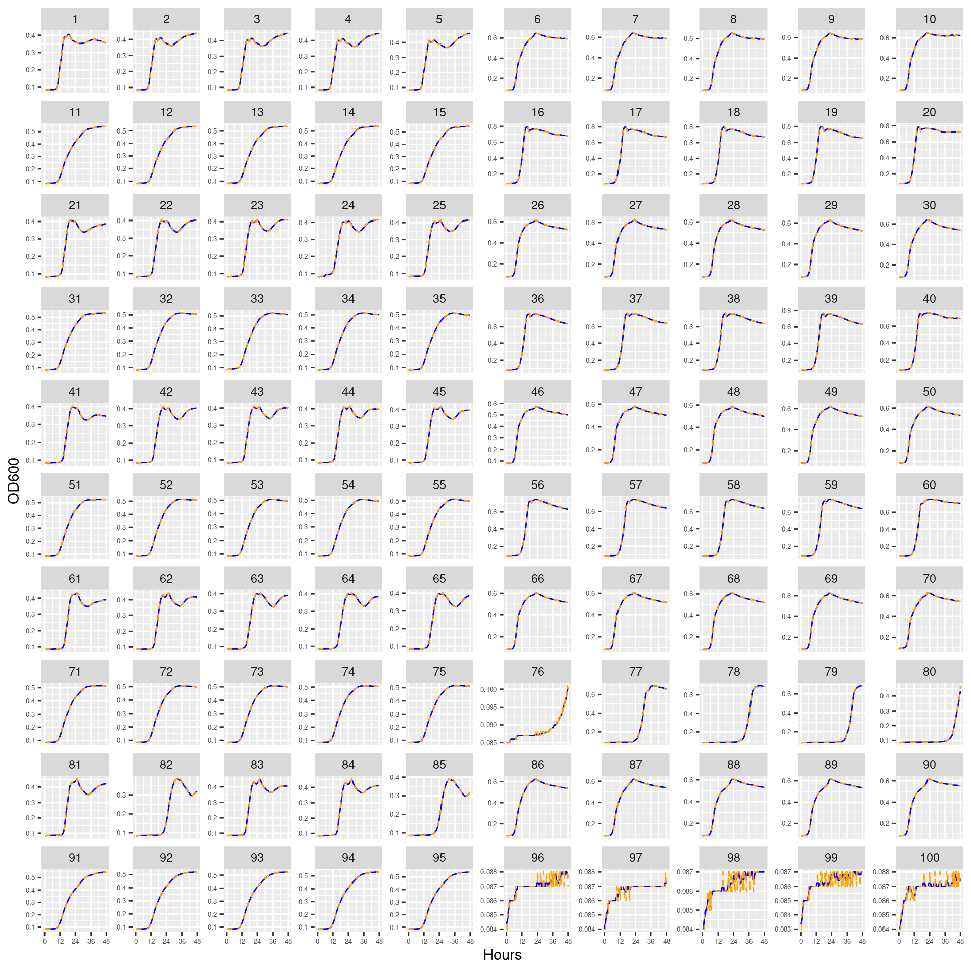
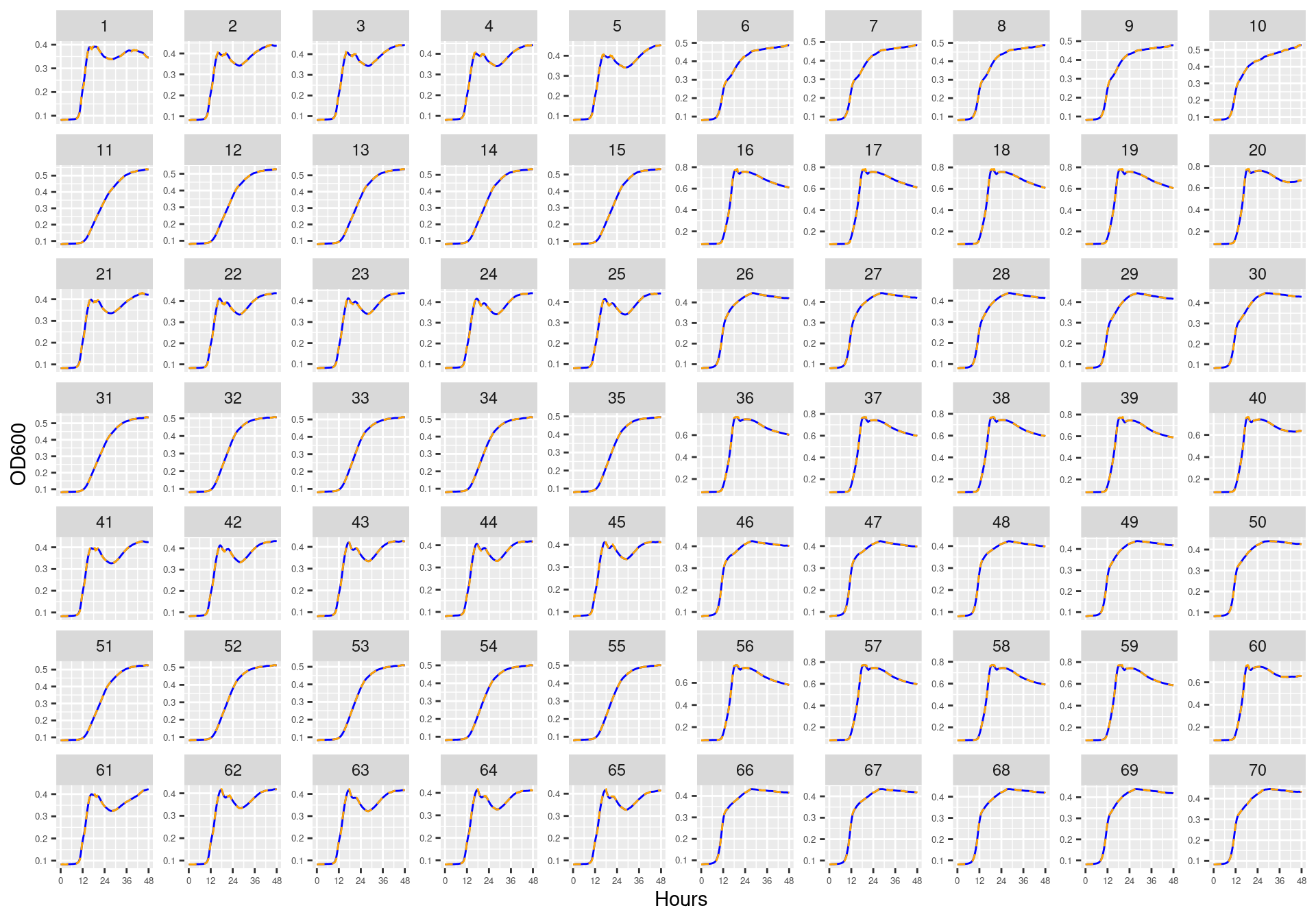
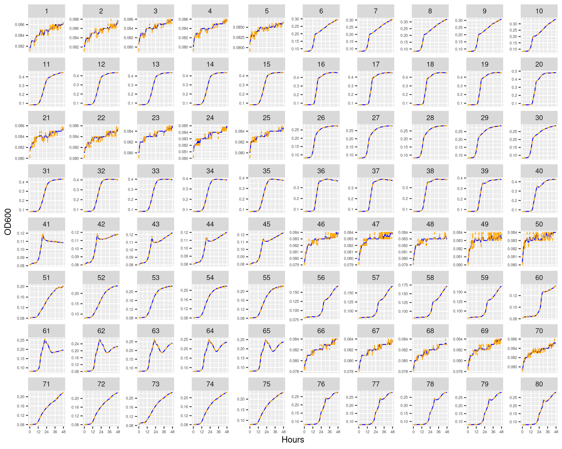
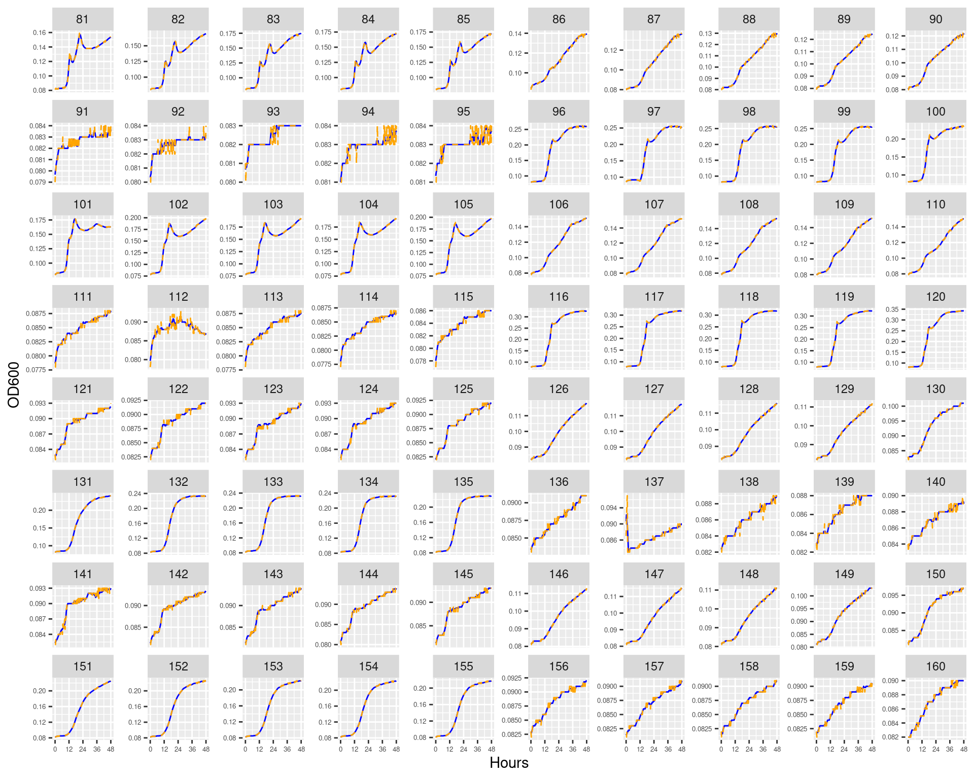
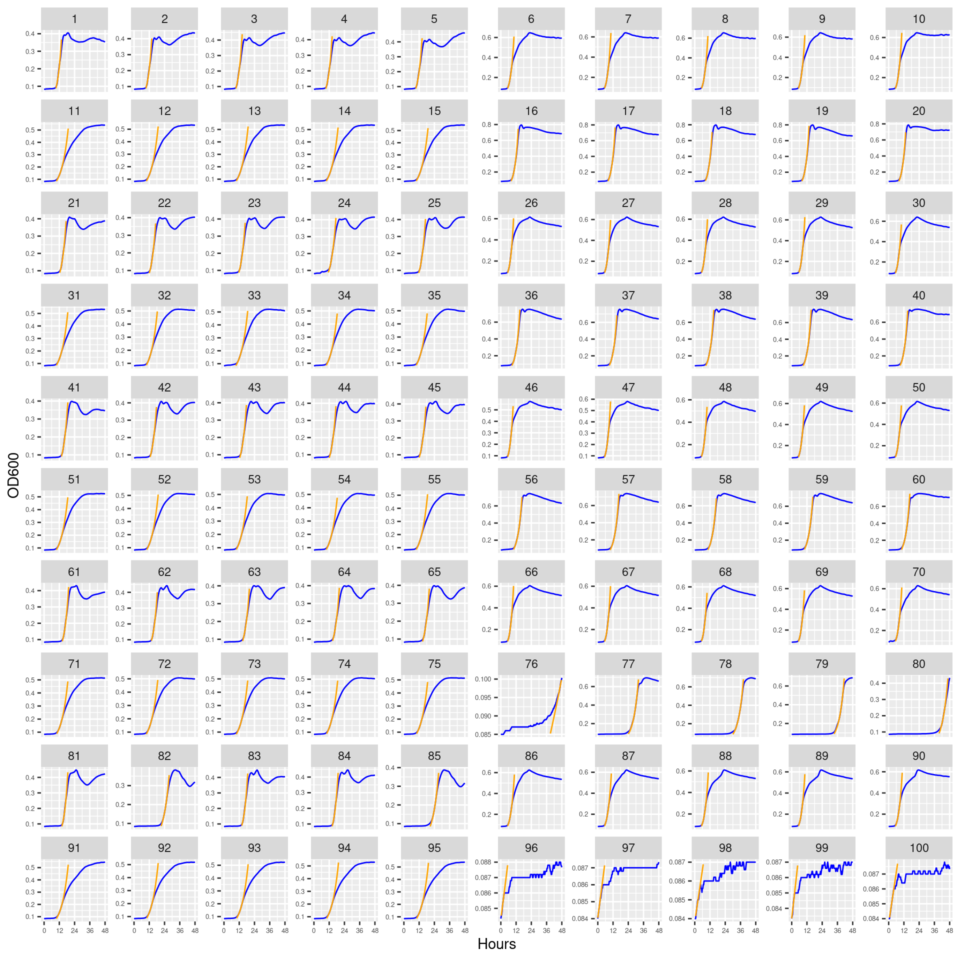
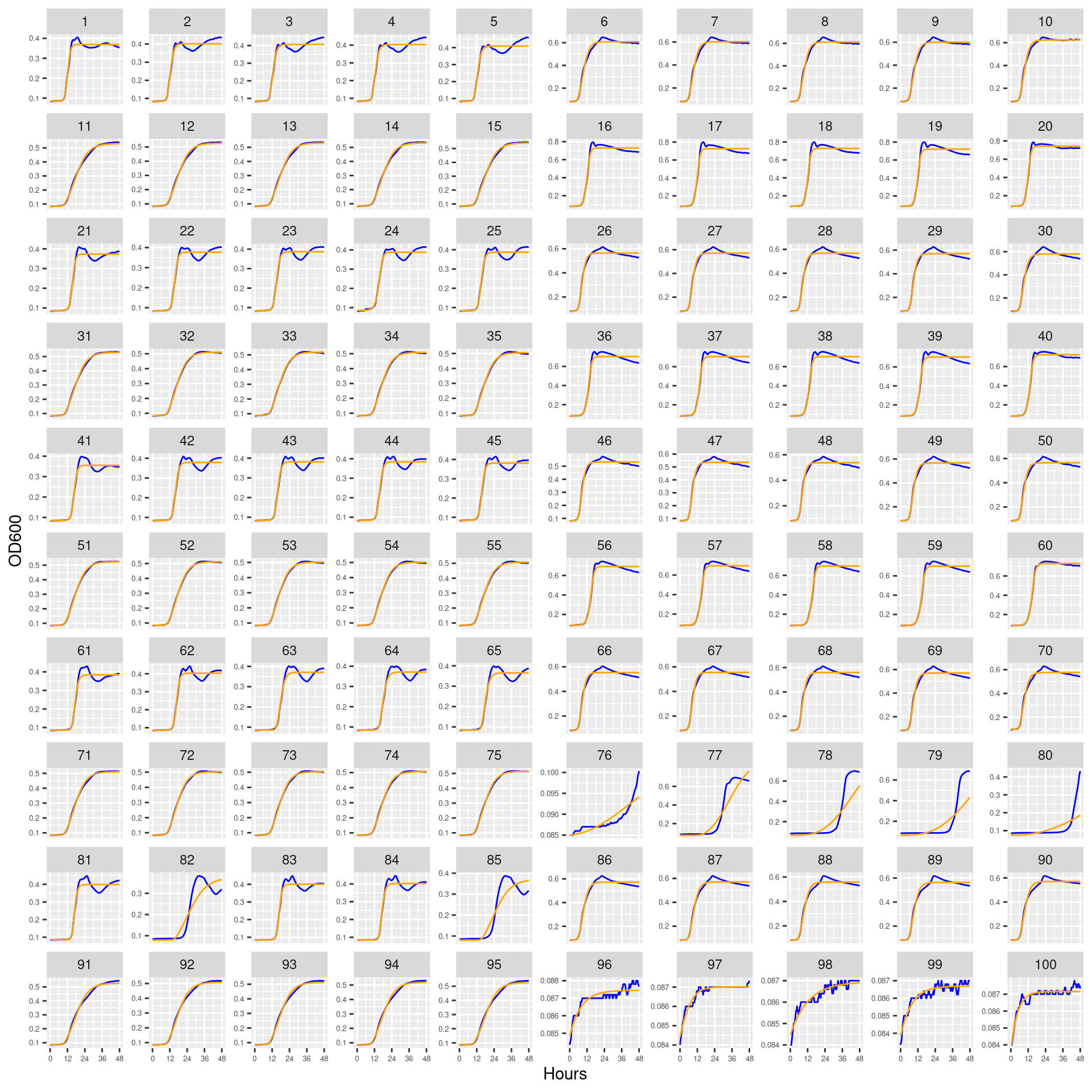
Figure 1: Bioscreen plate “bioscreen_strep_01” wells 1-100. Blue line is smoothed with a moving average window of 9 points. Orange is non-smoothed
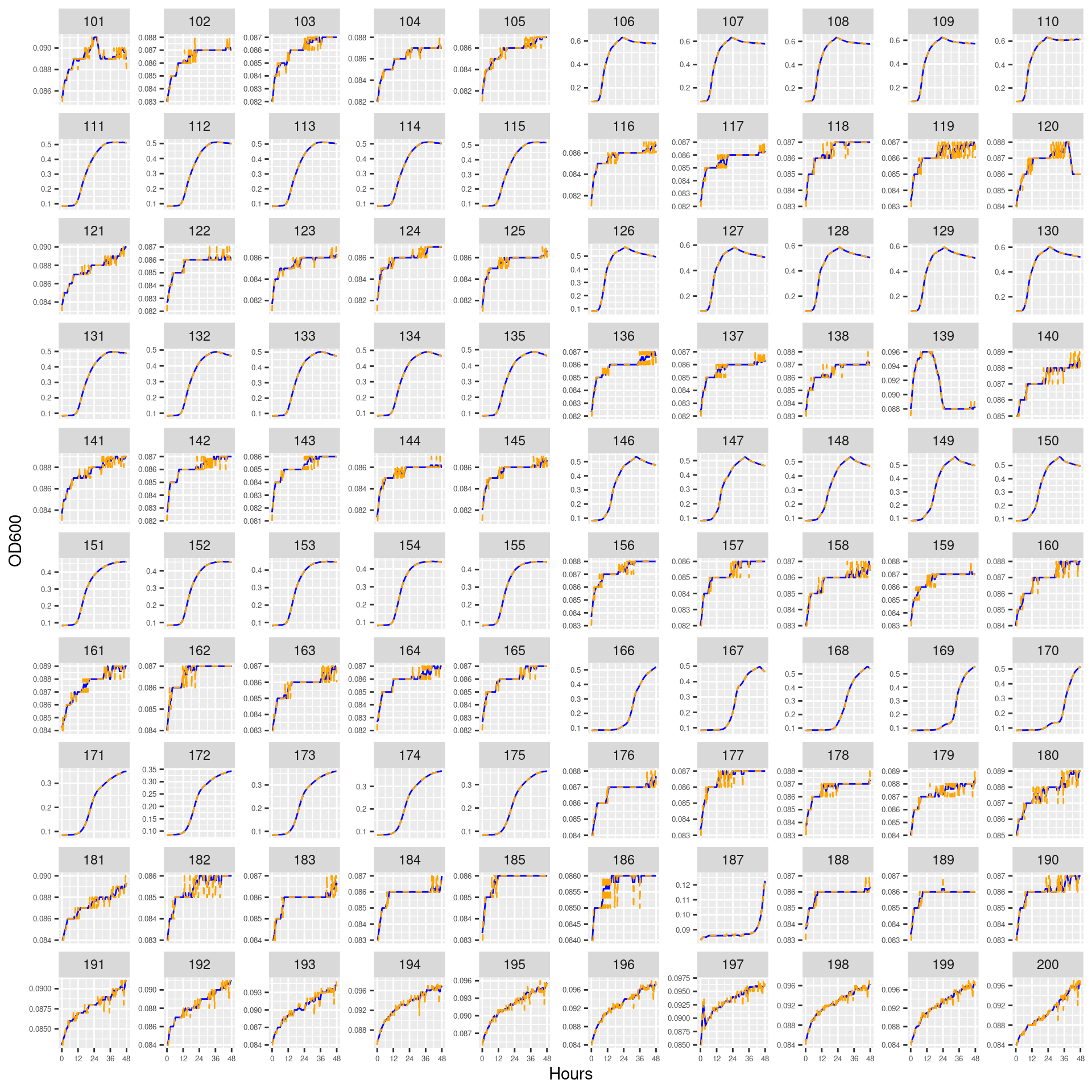
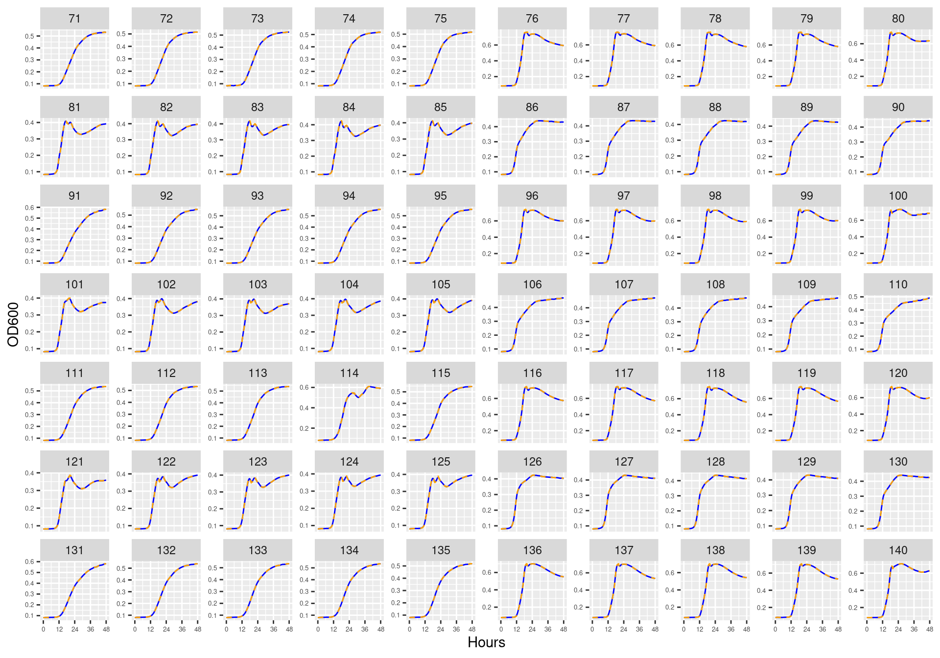
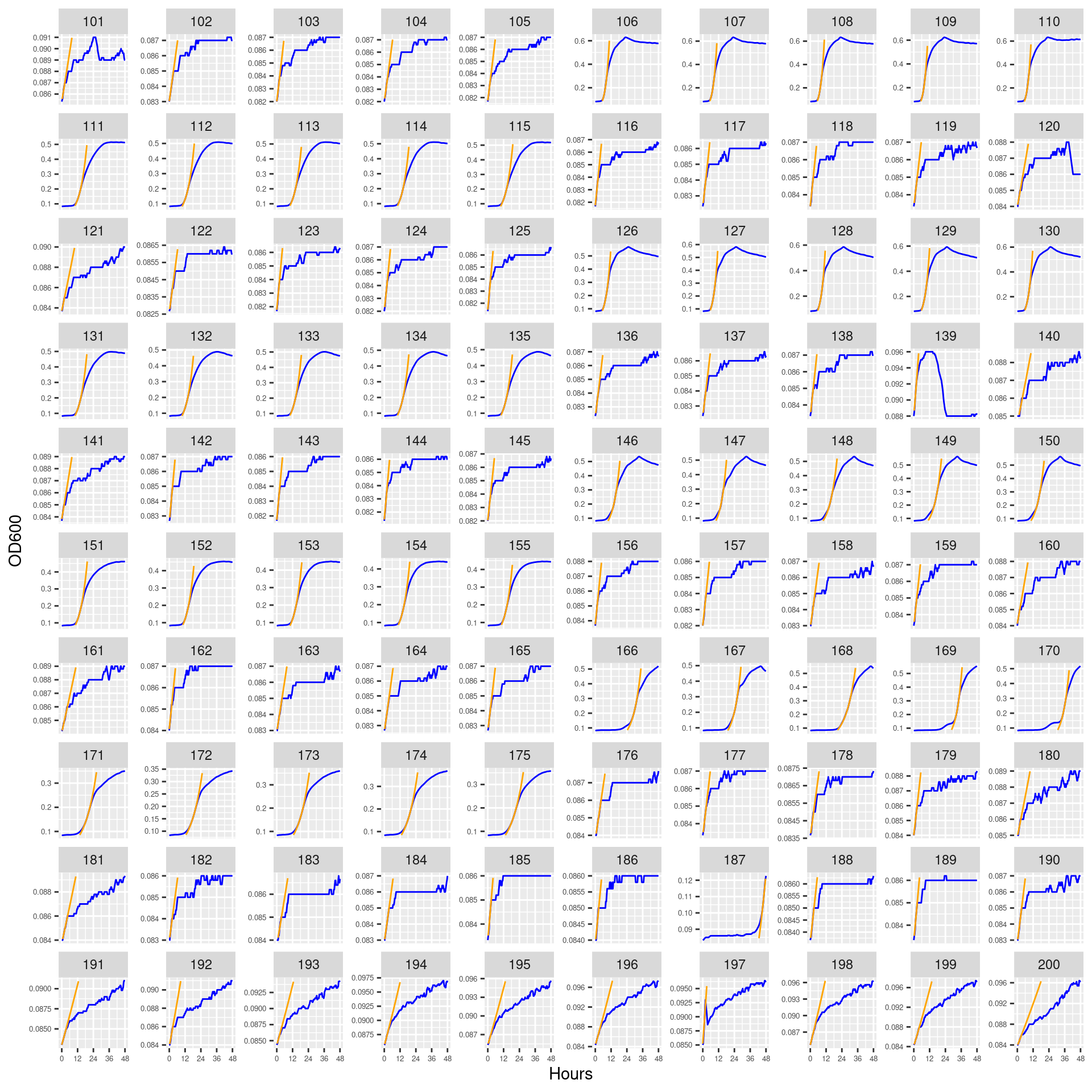
Figure 2: Bioscreen plate “bioscreen_strep_01” wells 101-200. Blue line is smoothed with a moving average window of 9 points. Orange is non-smoothed
5.2 bioscreen_strep_02
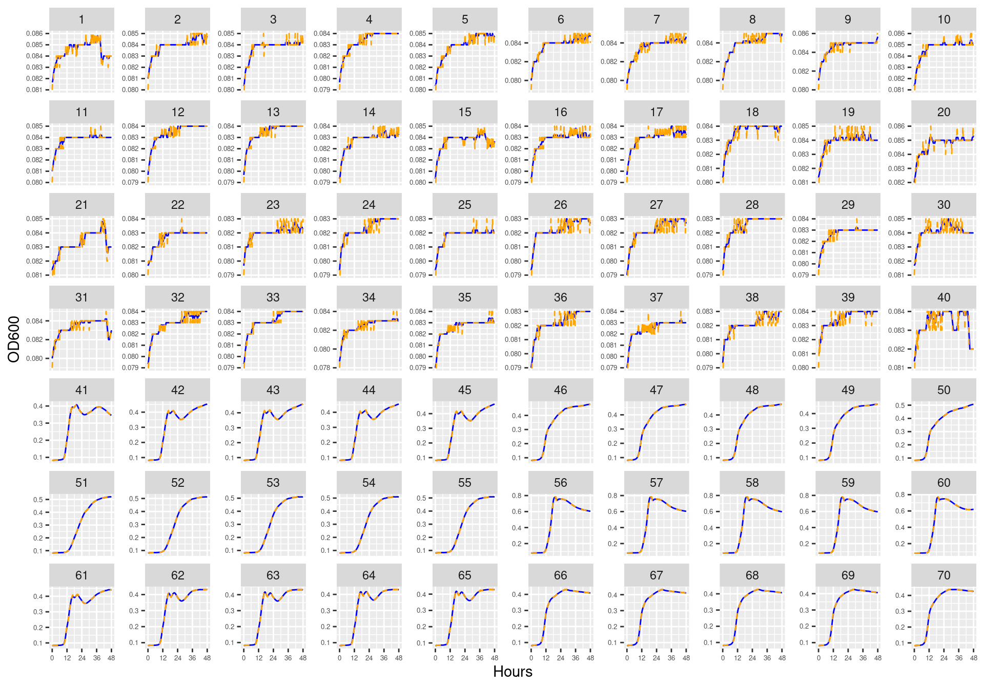
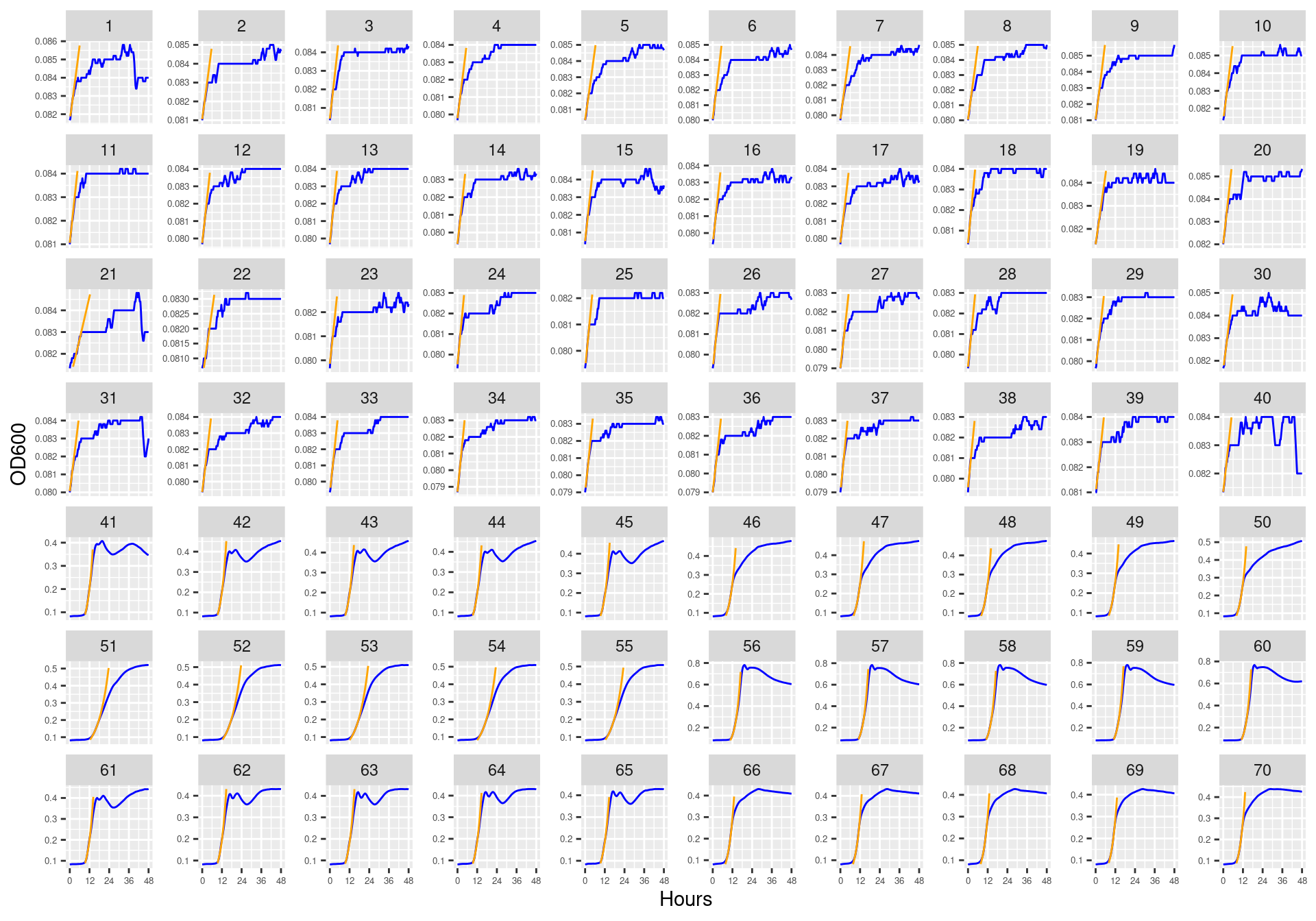
Figure 3: Bioscreen plate “bioscreen_strep_02” wells 1-70. Blue line is smoothed with a moving average window of 9 points. Orange is non-smoothed
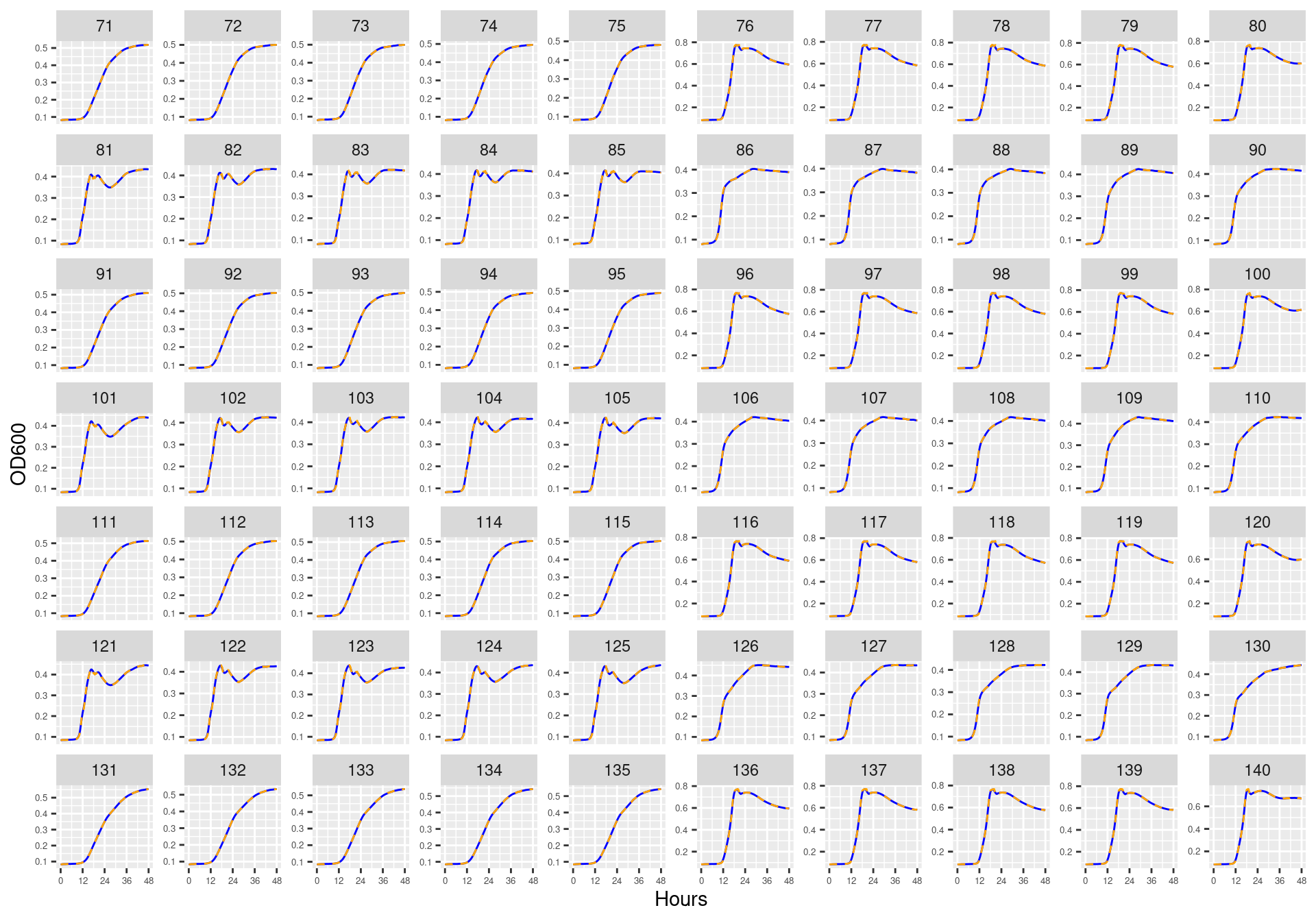
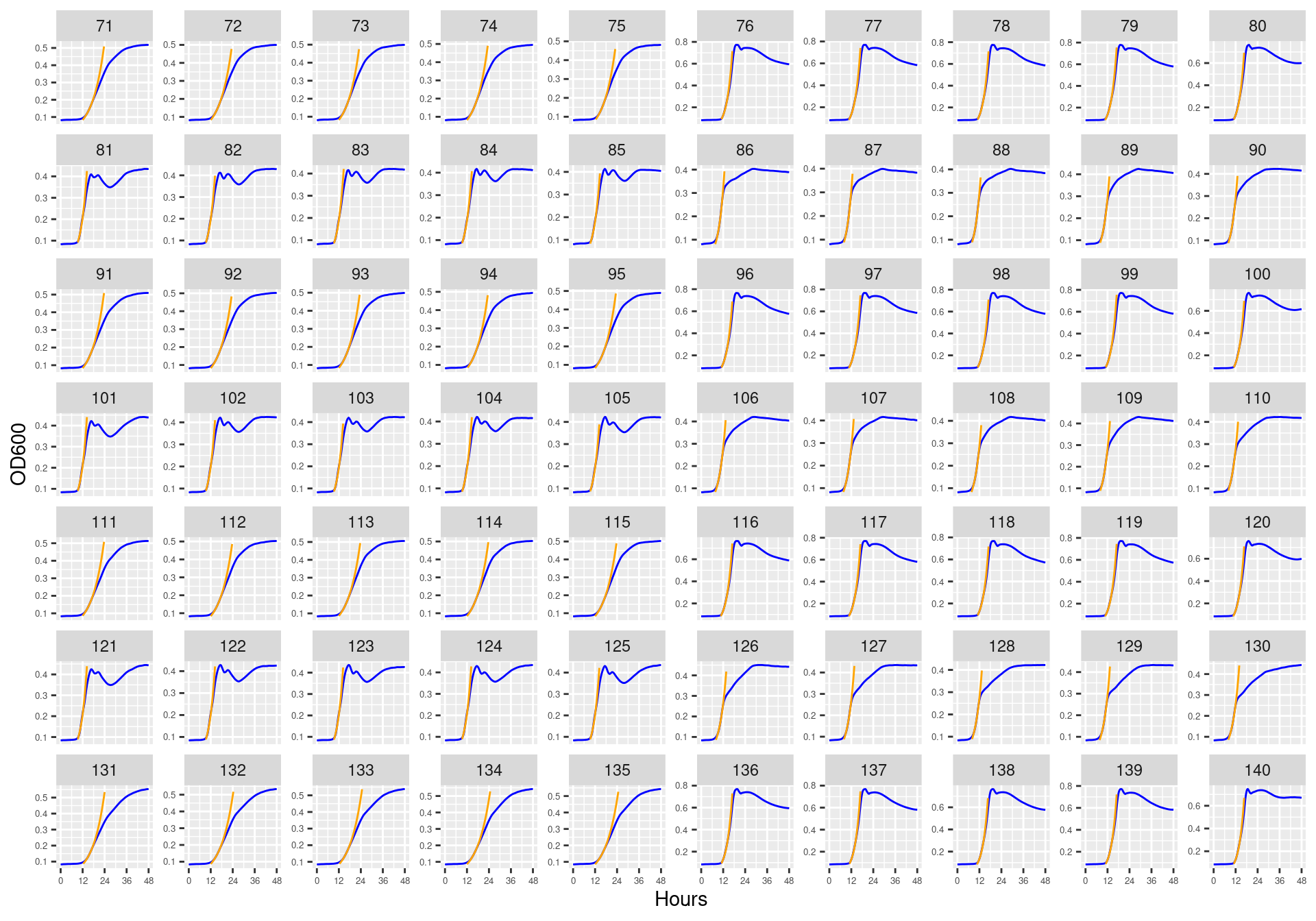
Figure 4: Bioscreen plate “bioscreen_strep_02” wells 71-140. Blue line is smoothed with a moving average window of 9 points. Orange is non-smoothed
5.3 bioscreen_strep_03
Figure 5: Bioscreen plate “bioscreen_strep_03” wells 1-70 Blue line is smoothed with a moving average window of 9 points. Orange is non-smoothed
Figure 6: Bioscreen plate “bioscreen_strep_03” wells 71-140. Blue line is smoothed with a moving average window of 9 points. Orange is non-smoothed
5.4 bioscreen_pairwise_filtrates_01
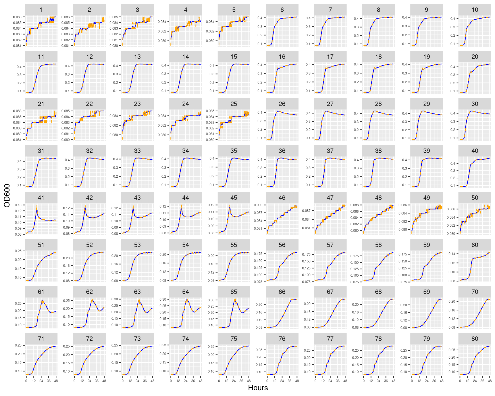
Figure 7: Bioscreen plate “bioscreen_pairwise_filtrates_01” wells 1-80 Blue line is smoothed with a moving average window of 9 points. Orange is non-smoothed
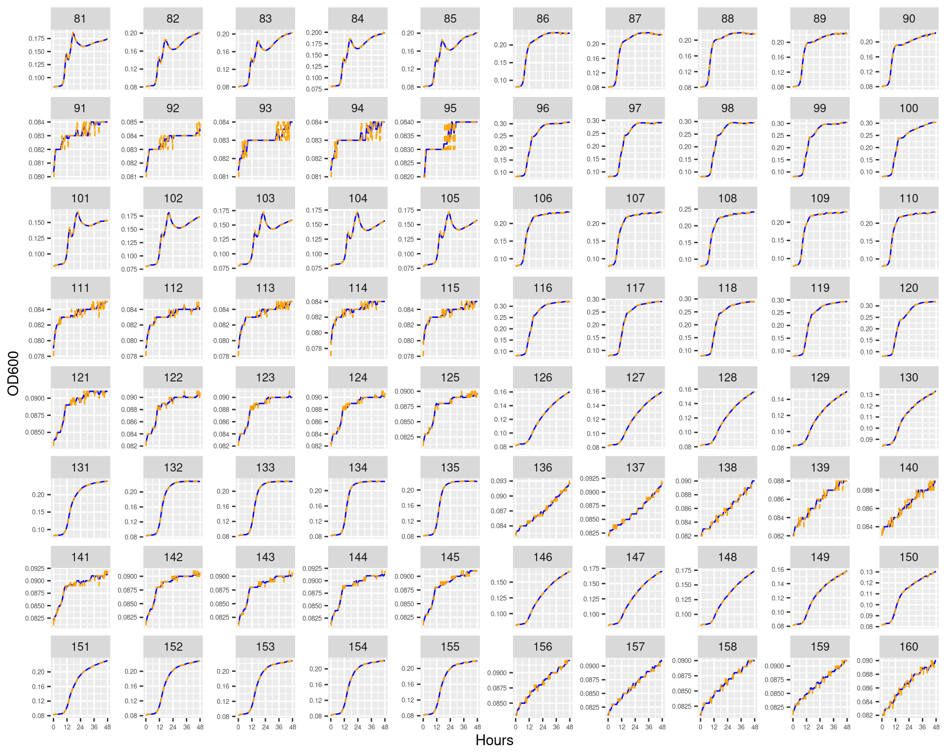
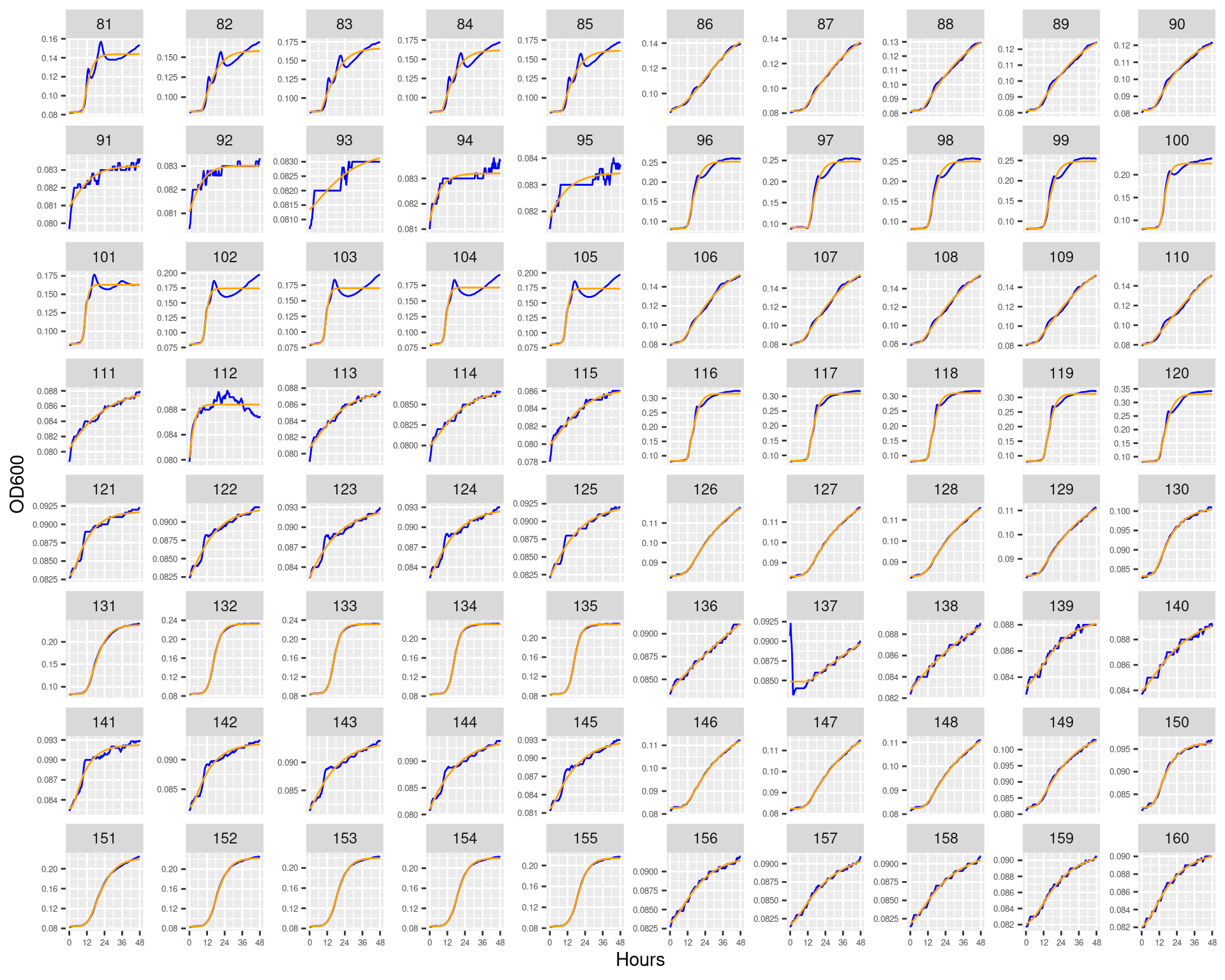
Figure 8: Bioscreen plate “bioscreen_pairwise_filtrates_01” wells 81-160 Blue line is smoothed with a moving average window of 9 points. Orange is non-smoothed
5.5 bioscreen_pairwise_filtrates_02
Figure 9: Bioscreen plate “bioscreen_pairwise_filtrates_02” wells 1-80. Blue line is smoothed with a moving average window of 9 points. Orange is non-smoothed
Figure 10: Bioscreen plate “bioscreen_pairwise_filtrates_02” wells 81-160. Blue line is smoothed with a moving average window of 9 points. Orange is non-smoothed
5.6 Conclusions
Growth curves all look reasonable. Can proceed with the analysis.
6 Growth curve statistics
Show/hide code
library("growthrates")
Loading required package: lattice
Loading required package: deSolve
Show/hide code
library("DescTools")
Attaching package: 'DescTools'
The following object is masked _by_ '.GlobalEnv':

    %nin%
gcurves_thin_sm <- gcurves_thin_sm %>%# make uniq idmutate(id =paste0(plate_name, "|", bioscreen_well))
6.1 Spline based estiamte
Smoothing splines are a quick method to estimate maximum growth. The method is called nonparametric, because the growth rate is directly estimated from the smoothed data without being restricted to a specific model formula.
The method was inspired by an algorithm of Kahm et al. (2010), with different settings and assumptions. In the moment, spline fitting is always done with log-transformed data, assuming exponential growth at the time point of the maximum of the first derivative of the spline fit. All the hard work is done by function smooth.spline from package stats, that is highly user configurable. Normally, smoothness is automatically determined via cross-validation. This works well in many cases, whereas manual adjustment is required otherwise, e.g. by setting spar to a fixed value [0, 1] that also disables cross-validation.
many_spline_xy <- purrr::map(many_spline@fits, \(x) data.frame(x = x@xy[1], y = x@xy[2])) %>% purrr::list_rbind(names_to ="id") %>% dplyr::mutate(id = stringr::str_remove_all(id, "bioscreen_pairwise_|bioscreen_"))many_spline_fitted <- purrr::map(many_spline@fits, \(x) data.frame(x@FUN(x@obs$time, x@par))) %>% purrr::list_rbind(names_to ="id") %>% dplyr::rename(hours = time, predicted = y) %>% dplyr::left_join(gcurves_thin_sm, by = dplyr::join_by(id, hours)) %>% dplyr::mutate(id = stringr::str_remove_all(id, "bioscreen_pairwise_|bioscreen_")) %>% dplyr::group_by(id) %>%# this step makes sure we don't plot fits that go outside the range of the data dplyr::mutate(predicted = dplyr::if_else(dplyr::between(predicted, min(OD600_rollmean), max(OD600_rollmean)), predicted, NA_real_)) %>% dplyr::ungroup()
6.1.4 Plot
6.1.4.1 bioscreen_strep_01
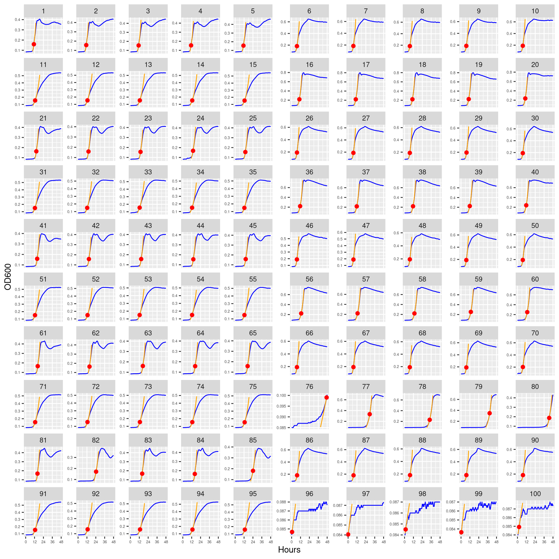
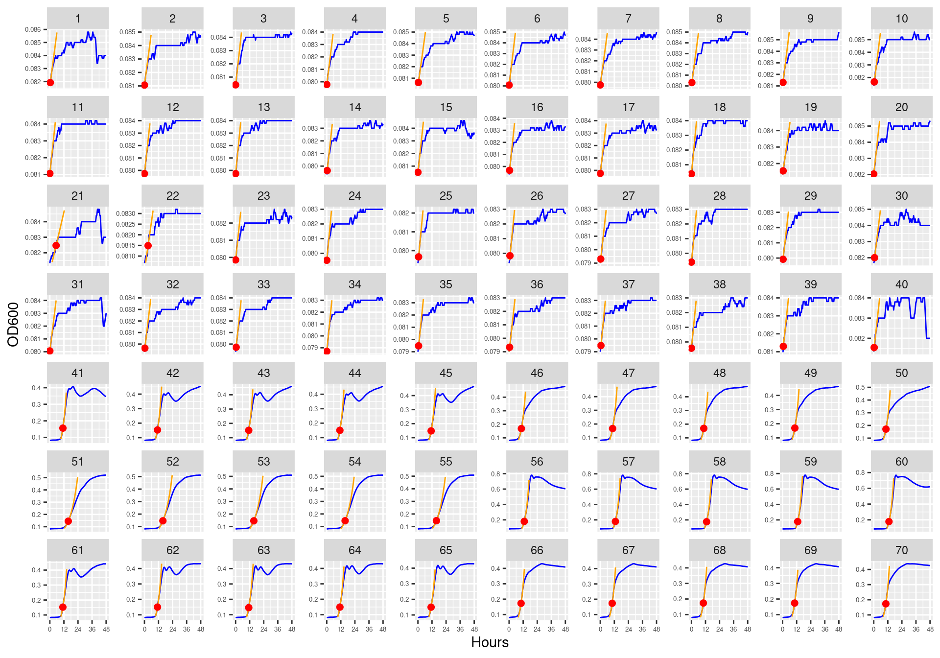
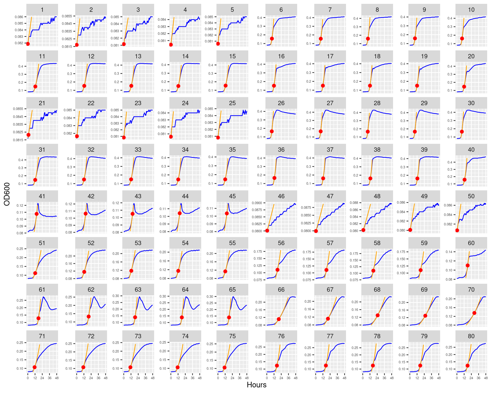
Figure 11: Bioscreen plate “bioscreen_strep_01” wells 1-100. Blue line is smoothed with a moving average window of 5 points. Orange is slope of max predicted growth rate from the first derivative of a smoothing spline. Red dot is hours and OD600 at which maximum growth rate is reached.
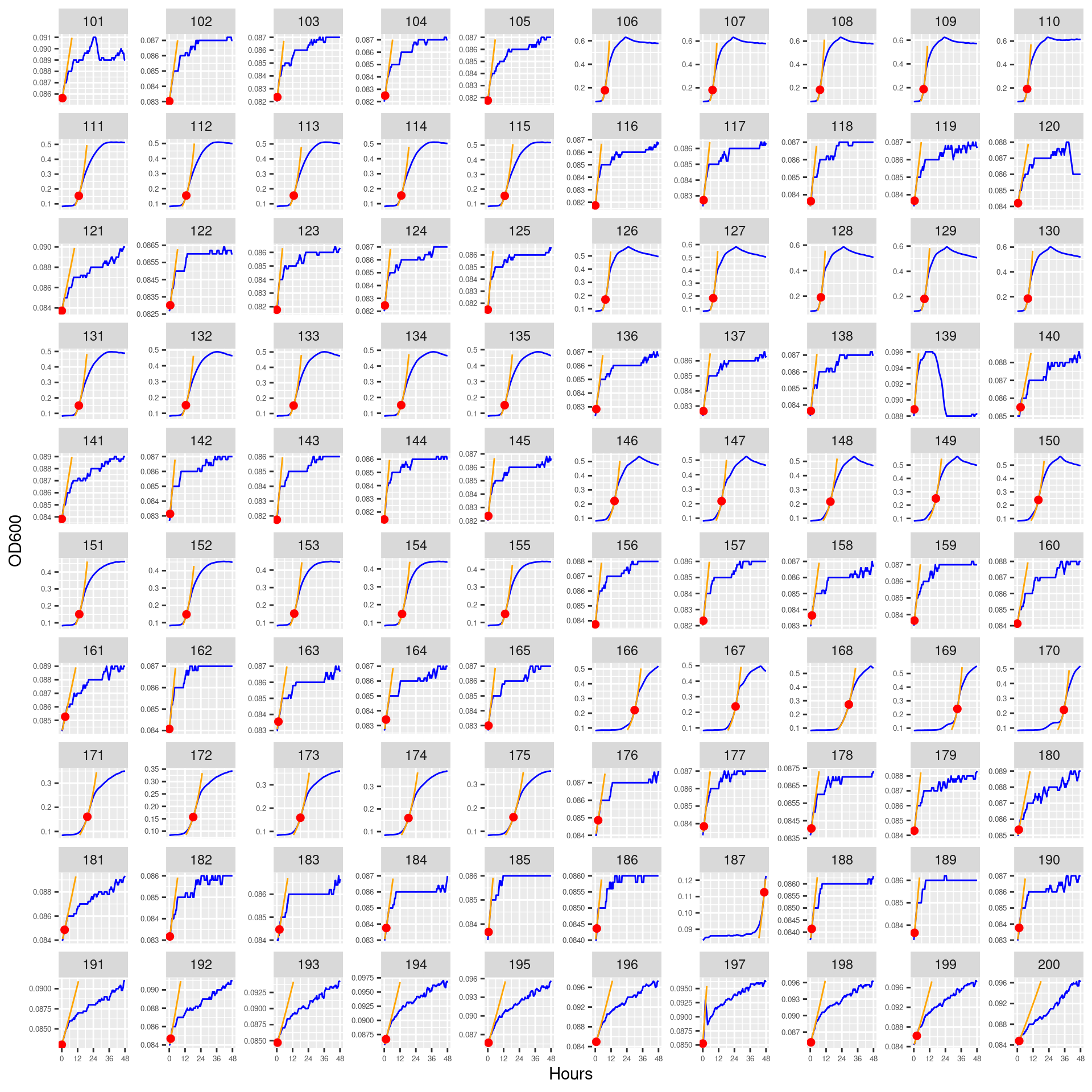
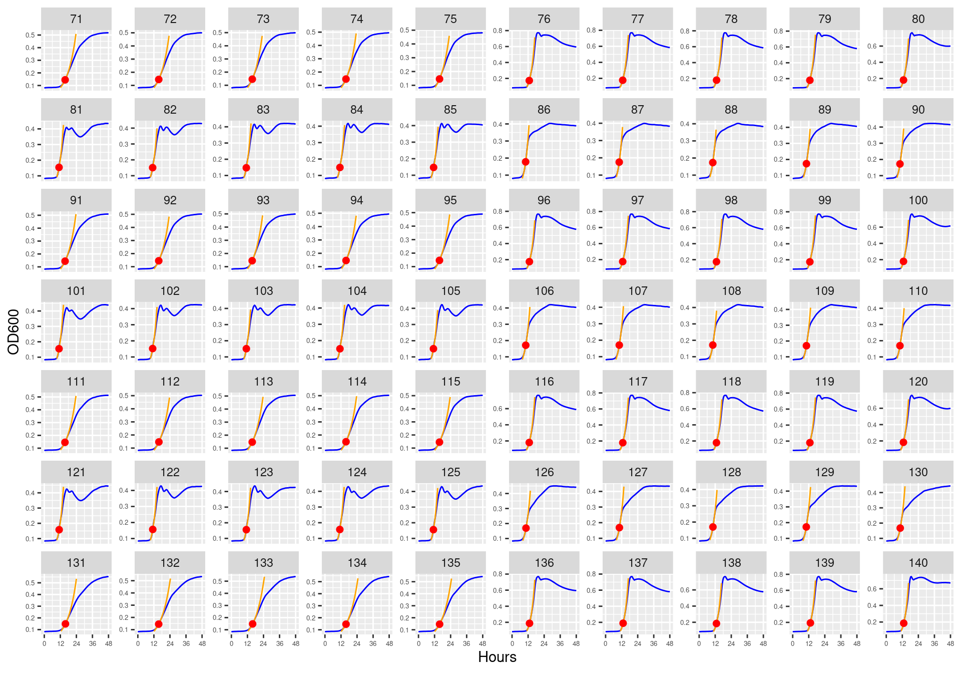
Figure 12: Bioscreen plate “bioscreen_strep_01” wells 101-200. Blue line is smoothed with a moving average window of 5 points. Orange is slope of max predicted growth rate from the first derivative of a smoothing spline. Red dot is hours and OD600 at which maximum growth rate is reached.
6.1.4.2 bioscreen_strep_02
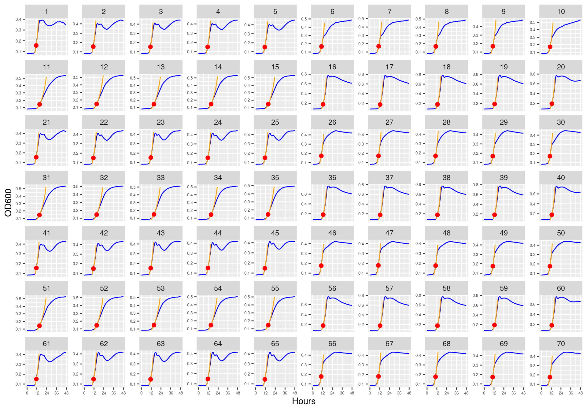
Figure 13: Bioscreen plate “bioscreen_strep_02” wells 1-70. Blue line is smoothed with a moving average window of 5 points. Orange is slope of max predicted growth rate from the first derivative of a smoothing spline. Red dot is hours and OD600 at which maximum growth rate is reached.
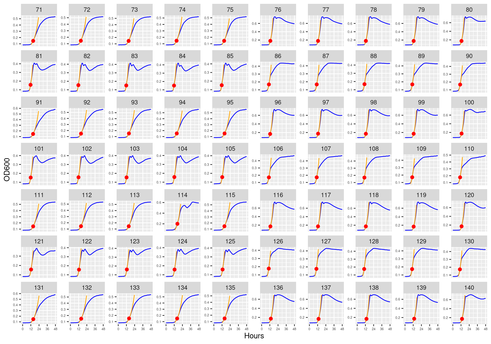
Figure 14: Bioscreen plate “bioscreen_strep_02” wells 71-140. Blue line is smoothed with a moving average window of 5 points. Orange is slope of max predicted growth rate from the first derivative of a smoothing spline. Red dot is hours and OD600 at which maximum growth rate is reached.
6.1.4.3 bioscreen_strep_03
Figure 15: Bioscreen plate “bioscreen_strep_03” wells 1-70. Blue line is smoothed with a moving average window of 5 points. Orange is slope of max predicted growth rate from the first derivative of a smoothing spline. Red dot is hours and OD600 at which maximum growth rate is reached.
Figure 16: Bioscreen plate “bioscreen_strep_03” wells 71-140. Blue line is smoothed with a moving average window of 5 points. Orange is slope of max predicted growth rate from the first derivative of a smoothing spline. Red dot is hours and OD600 at which maximum growth rate is reached.
6.1.4.4 bioscreen_pairwise_filtrates_01
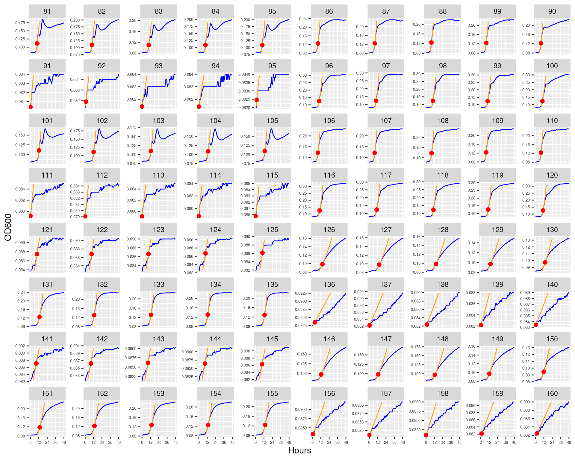
Figure 17: Bioscreen plate “bioscreen_pairwise_filtrates_01” wells 1-80. Blue line is smoothed with a moving average window of 5 points. Orange is slope of max predicted growth rate. Red dot is hours and OD600 at which maximum growth rate is reached.
Figure 18: Bioscreen plate “bioscreen_pairwise_filtrates_01” wells 81-160. Blue line is smoothed with a moving average window of 5 points. Orange is slope of max predicted growth rate. Red dot is hours and OD600 at which maximum growth rate is reached.
6.1.4.5 bioscreen_pairwise_filtrates_02
Figure 19: Bioscreen plate “bioscreen_pairwise_filtrates_02” wells 1-80. Blue line is smoothed with a moving average window of 5 points. Orange is slope of max predicted growth rate. Red dot is hours and OD600 at which maximum growth rate is reached.
Figure 20: Bioscreen plate “bioscreen_pairwise_filtrates_02” wells 81-160. Blue line is smoothed with a moving average window of 5 points. Orange is slope of max predicted growth rate. Red dot is hours and OD600 at which maximum growth rate is reached.
6.2 Linear model based estimate
This method determine maximum growth rates from the log-linear part of a growth curve using a heuristic approach similar to the “growth rates made easy” method of Hall et al. (2013).
1. Fit linear regressions to all subsets of h consecutive data points. If for example h = 5, fit a linear regression to points 1 . . . 5, 2 . . . 6, 3. . . 7 and so on. The method seeks the highest rate of exponential growth, so the dependent variable is of course log-transformed.
2. Find the subset with the highest slope bmax and include also the data points of adjacent subsets that have a slope of at least quota · bmax, e.g. all data sets that have at least 95% of the maximum slope.
3. Fit a new linear model to the extended data window identified in step 2.
many_linear_fitted <- purrr::map(many_spline@fits, \(x) data.frame(x@FUN(x@obs$time, x@par))) %>% purrr::list_rbind(names_to ="id") %>% dplyr::rename(hours = time, predicted = y) %>% dplyr::left_join(gcurves_thin_sm, by = dplyr::join_by(id, hours)) %>% dplyr::mutate(id = stringr::str_remove_all(id, "bioscreen_pairwise_|bioscreen_")) %>% dplyr::group_by(id) %>%# this step makes sure we don't plot fits that go outside the range of the data dplyr::mutate(predicted = dplyr::if_else(dplyr::between(predicted, min(OD600_rollmean), max(OD600_rollmean)), predicted, NA_real_)) %>% dplyr::ungroup()
6.2.4 Plot
6.2.4.1 bioscreen_strep_01
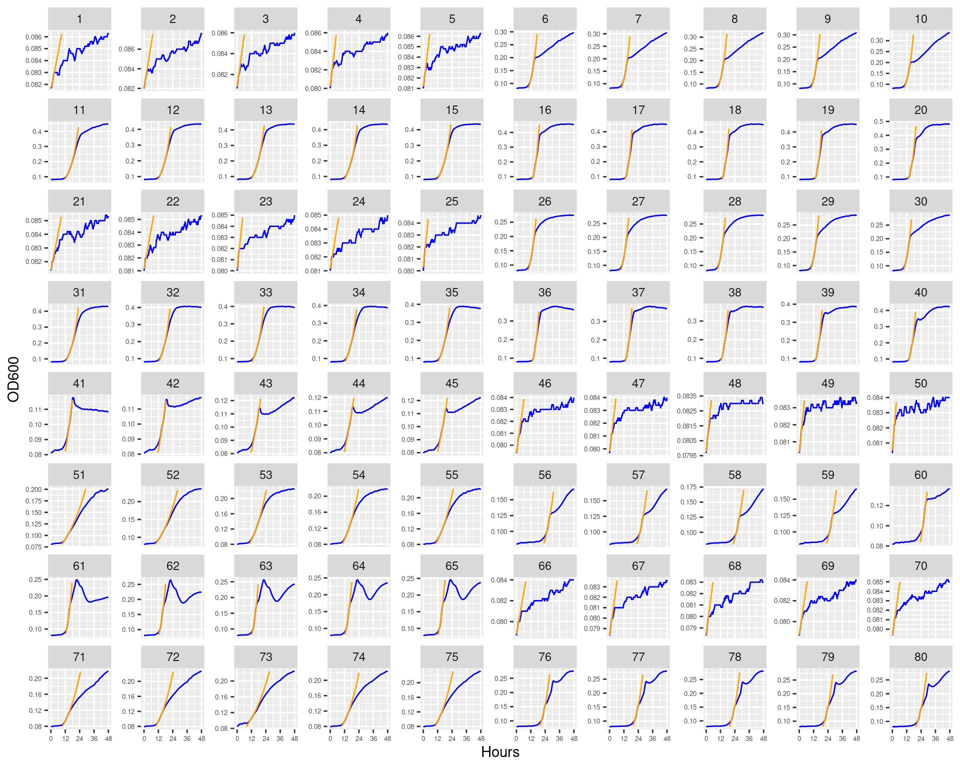
Figure 21: Bioscreen plate “bioscreen_strep_01” wells 1-100. Blue line is smoothed with a moving average window of 5 points. Orange is slope of max predicted growth rate from a piecewise linear model fit.
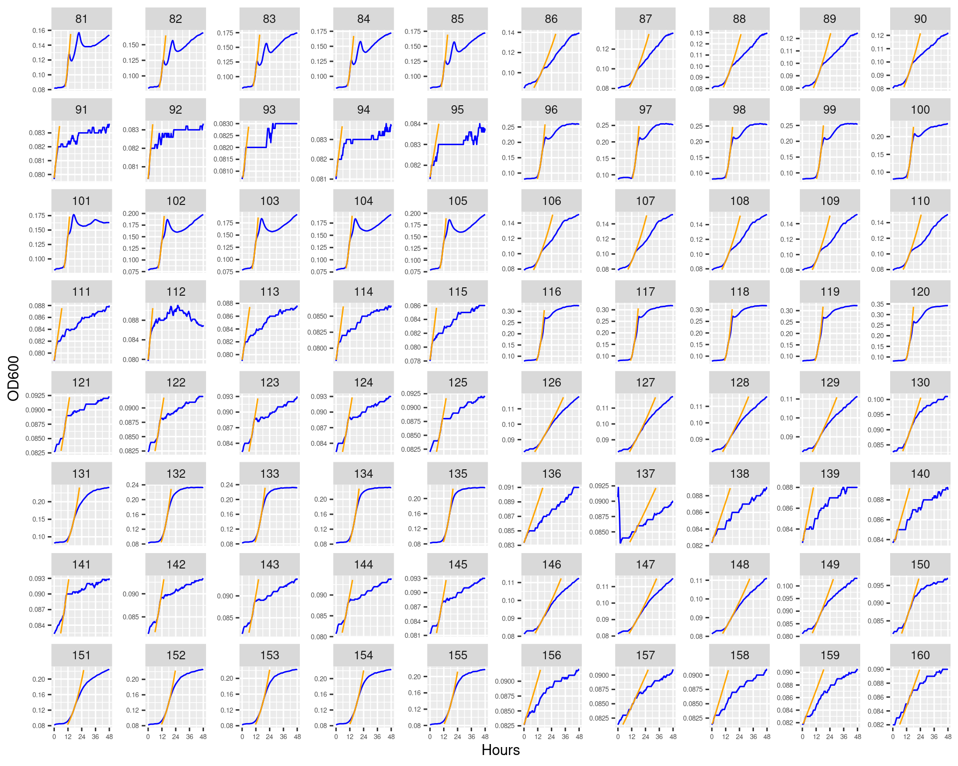
Figure 22: Bioscreen plate “bioscreen_strep_01” wells 101-200. Blue line is smoothed with a moving average window of 5 points. Orange is slope of max predicted growth rate from a piecewise linear model fit.
6.2.4.2 bioscreen_strep_02
Figure 23: Bioscreen plate “bioscreen_strep_02” wells 1-70. Blue line is smoothed with a moving average window of 5 points. Orange is slope of max predicted growth rate from a piecewise linear model fit.
Figure 24: Bioscreen plate “bioscreen_strep_02” wells 71-140. Blue line is smoothed with a moving average window of 5 points. Orange is slope of max predicted growth rate from a piecewise linear model fit.
6.2.4.3 bioscreen_strep_03
Figure 25: Bioscreen plate “bioscreen_strep_03” wells 1-70. Blue line is smoothed with a moving average window of 5 points. Orange is slope of max predicted growth rate from a piecewise linear model fit.
Figure 26: Bioscreen plate “bioscreen_strep_03” wells 71-140. Blue line is smoothed with a moving average window of 5 points. Orange is slope of max predicted growth rate from a piecewise linear model fit.
6.2.4.4 bioscreen_pairwise_filtrates_01
Figure 27: Bioscreen plate “bioscreen_pairwise_filtrates_01” wells 1-80. Blue line is smoothed with a moving average window of 5 points. Orange is slope of max predicted growth rate from a piecewise linear model fit.
Figure 28: Bioscreen plate “bioscreen_pairwise_filtrates_01” wells 81-160. Blue line is smoothed with a moving average window of 5 points. Orange is slope of max predicted growth rate from a piecewise linear model fit.
6.2.4.5 bioscreen_pairwise_filtrates_02
Figure 29: Bioscreen plate “bioscreen_pairwise_filtrates_02” wells 1-80. Blue line is smoothed with a moving average window of 5 points. Orange is slope of max predicted growth rate from a piecewise linear model fit.
Figure 30: Bioscreen plate “bioscreen_pairwise_filtrates_02” wells 81-160. Blue line is smoothed with a moving average window of 5 points. Orange is slope of max predicted growth rate from a piecewise linear model fit.
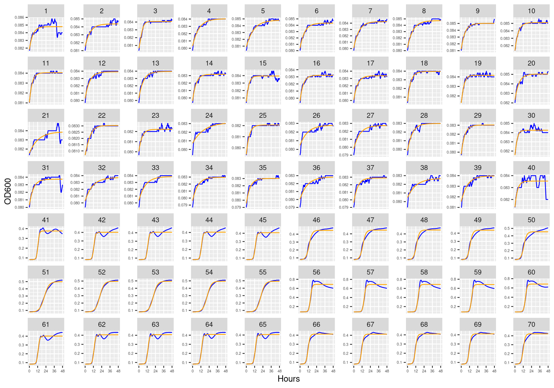
6.3 Baranyi parametric fit estimate
This uses the growth model of Baranyi and Roberts (1995) written as analytical solution of the system of differential equations.
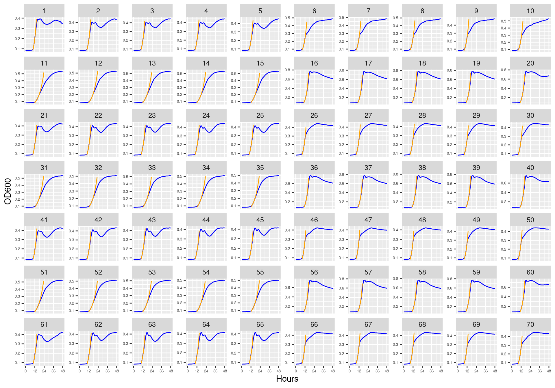
Figure 31: Bioscreen plate “bioscreen_strep_01” wells 1-100. Blue line is smoothed with a moving average window of 5 points. Orange is fitted to the Baranyi 1995 model.
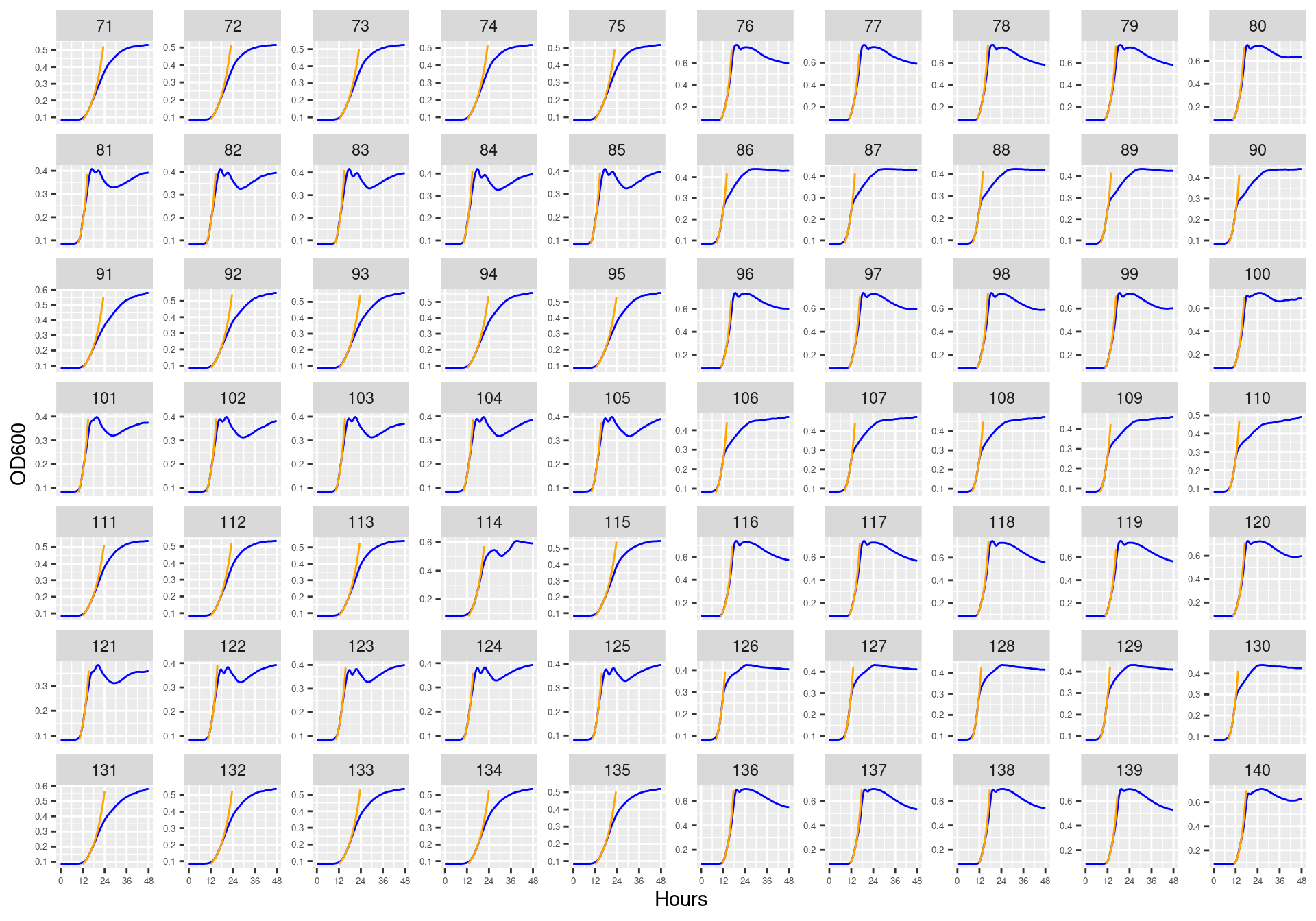
Figure 32: Bioscreen plate “bioscreen_strep_01” wells 101-200. Blue line is smoothed with a moving average window of 5 points. Orange is fitted to the Baranyi 1995 model.
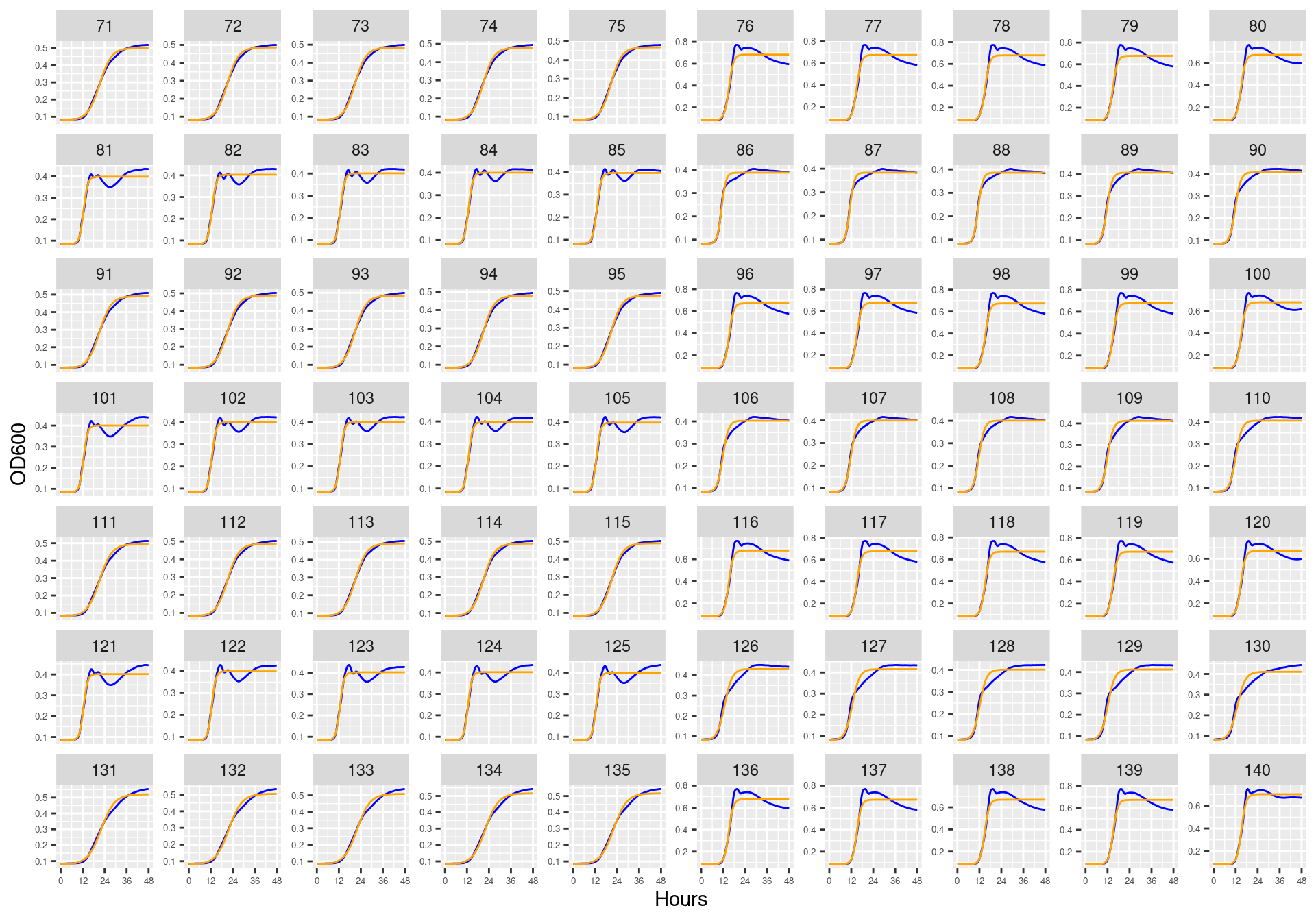
6.3.4.2 bioscreen_strep_02
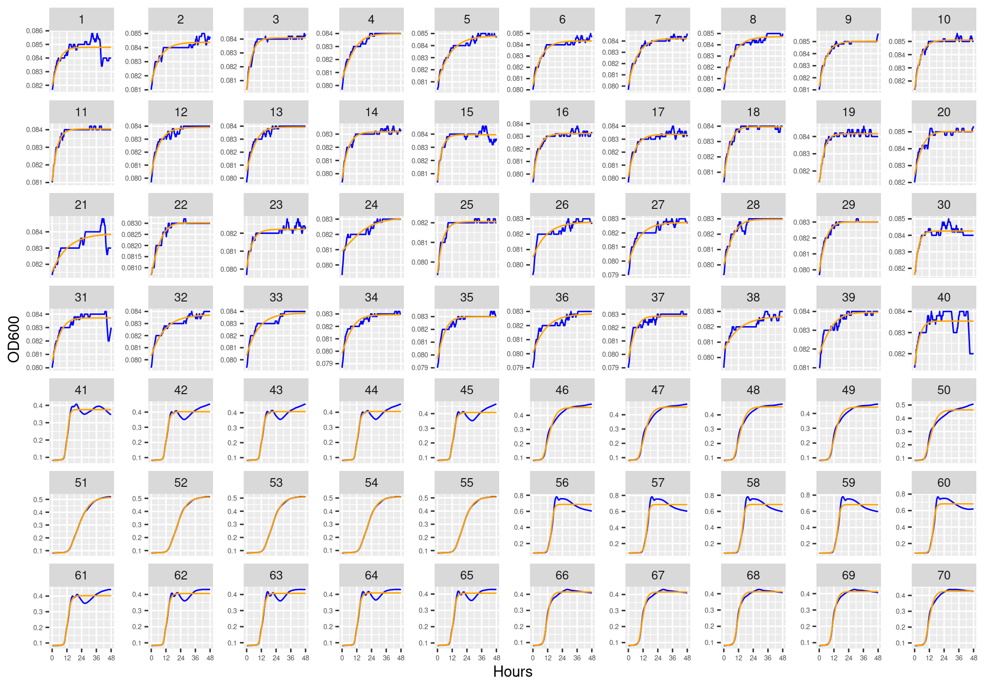
Figure 33: Bioscreen plate “bioscreen_strep_02” wells 1-70. Blue line is smoothed with a moving average window of 5 points. Orange is fitted to the Baranyi 1995 model.
Figure 34: Bioscreen plate “bioscreen_strep_02” wells 71-140. Blue line is smoothed with a moving average window of 5 points. Orange is fitted to the Baranyi 1995 model.
6.3.4.3 bioscreen_strep_03
Figure 35: Bioscreen plate “bioscreen_strep_03” wells 1-70. Blue line is smoothed with a moving average window of 5 points. Orange is fitted to the Baranyi 1995 model.
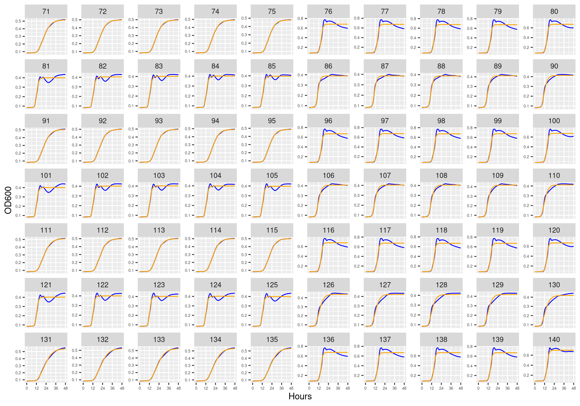
Figure 36: Bioscreen plate “bioscreen_strep_03” wells 71-140. Blue line is smoothed with a moving average window of 5 points. Orange is fitted to the Baranyi 1995 model.
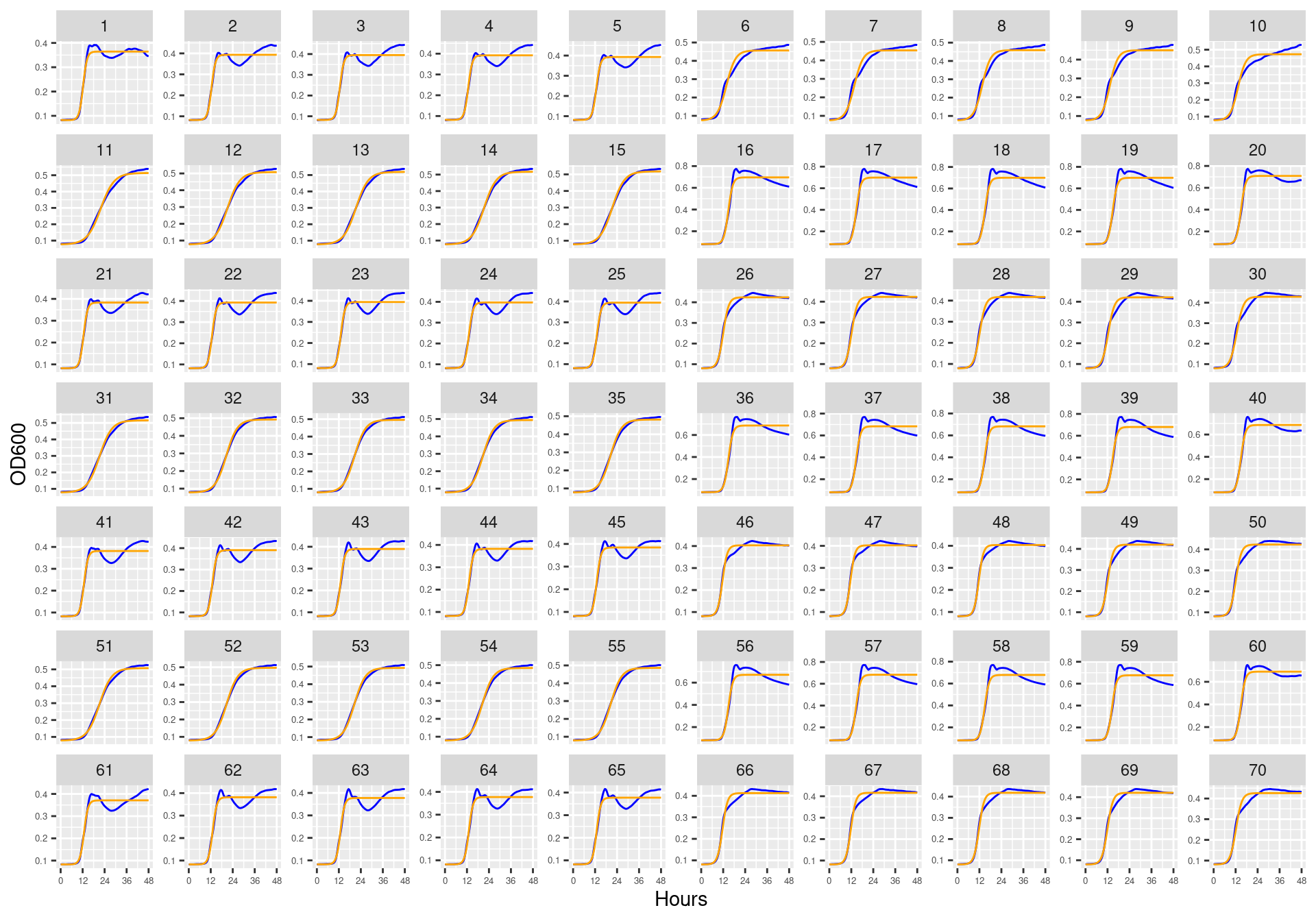
6.3.4.4 bioscreen_pairwise_filtrates_01
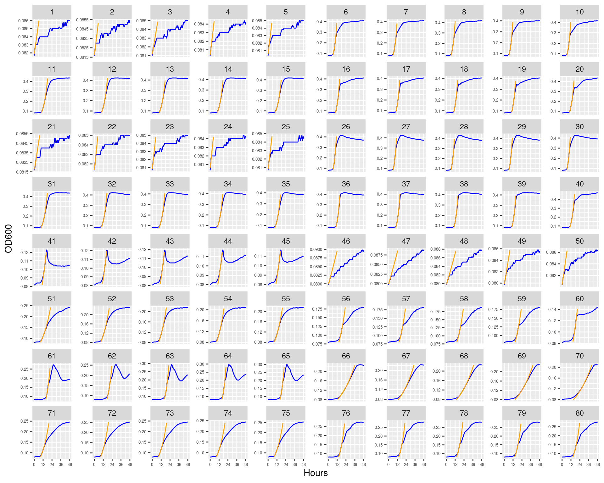
Figure 37: Bioscreen plate “bioscreen_pairwise_filtrates_01” wells 1-80. Blue line is smoothed with a moving average window of 5 points. Orange is fitted to the Baranyi 1995 model.
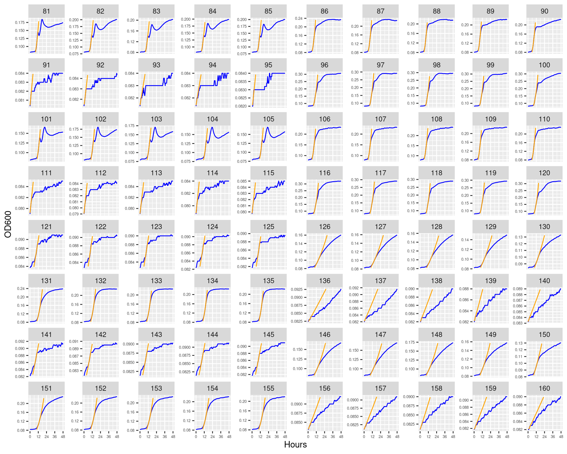
Figure 38: Bioscreen plate “bioscreen_pairwise_filtrates_01” wells 81-160. Blue line is smoothed with a moving average window of 5 points. Orange is fitted to the Baranyi 1995 model.
6.3.4.5 bioscreen_pairwise_filtrates_02
Figure 39: Bioscreen plate “bioscreen_pairwise_filtrates_02” wells 1-80. Blue line is smoothed with a moving average window of 5 points. Orange is fitted to the Baranyi 1995 model.
Figure 40: Bioscreen plate “bioscreen_pairwise_filtrates_02” wells 81-160. Blue line is smoothed with a moving average window of 5 points. Orange is fitted to the Baranyi 1995 model.
6.4 Huang parametric fit estimate
Huangs growth model (ref 1, ref 2) written as analytical solution of the differential equations.
In contrast to the original publication, all parameters related to population abundance (y, y0, K) are given as untransformed values. They are not log-transformed. In general, using log-transformed parameters would indeed be a good idea to avoid the need of constained optimization, but tests showed that box-constrained optimization worked resonably well. Therefore, handling of optionally log-transformed parameters was removed from the package to avoid confusion. If you want to discuss this, please let me know.
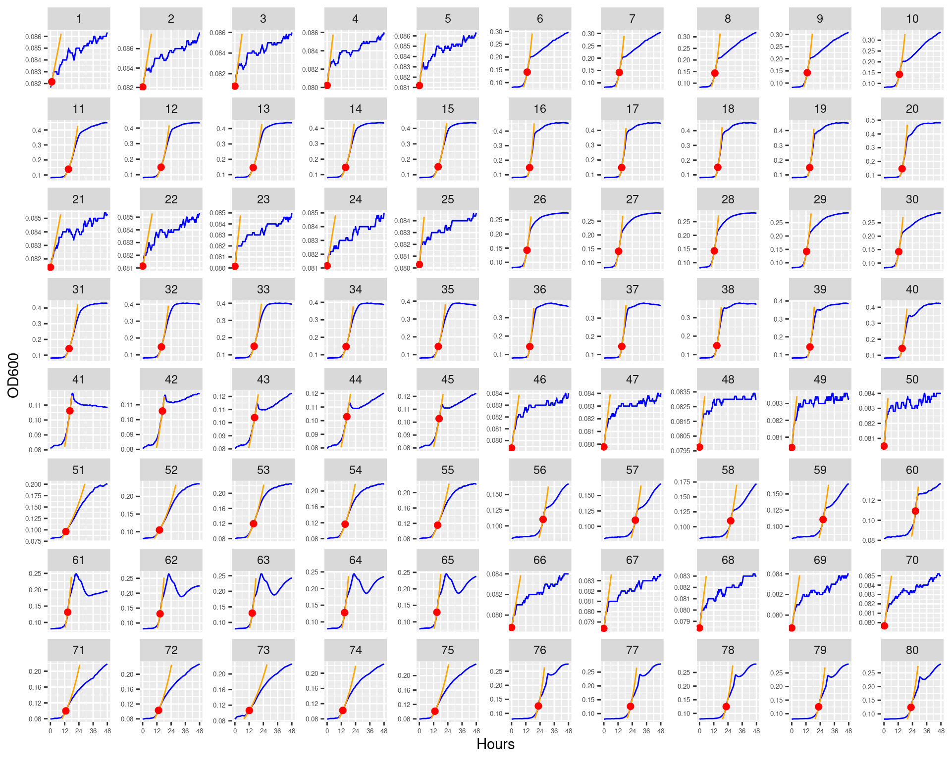
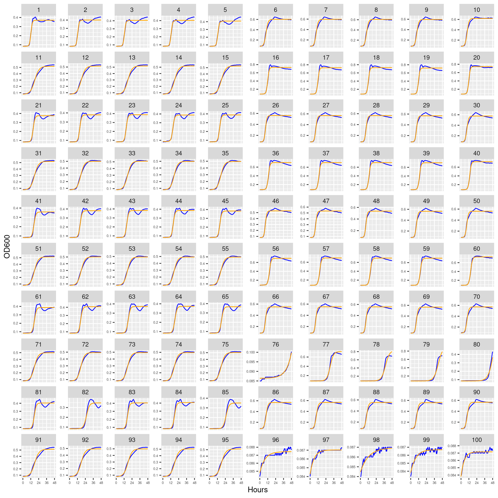
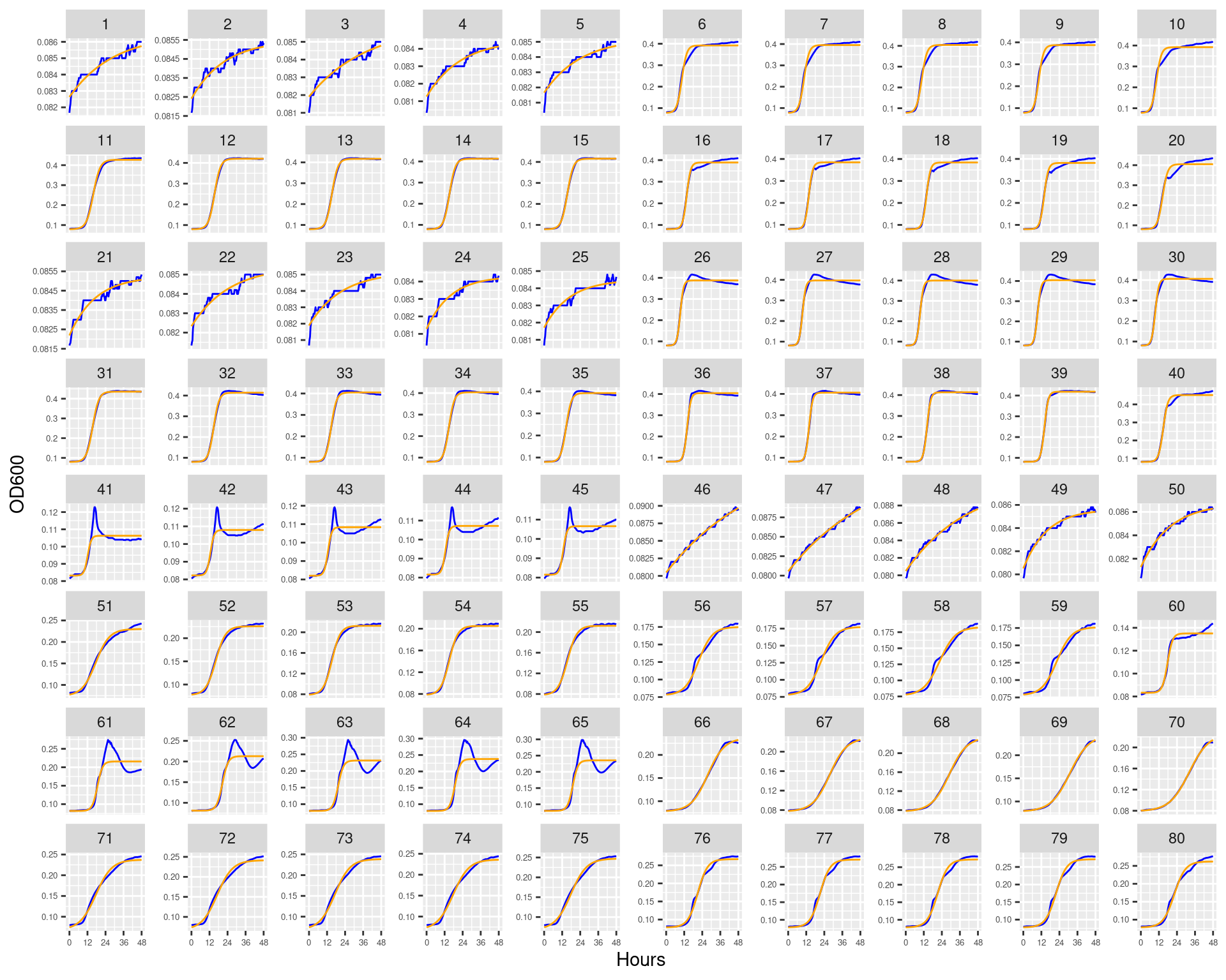
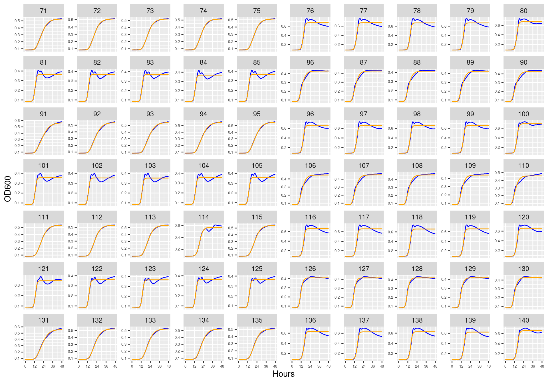
Figure 41: Bioscreen plate “bioscreen_strep_01” wells 1-100. Blue line is smoothed with a moving average window of 5 points. Orange is fitted to the Huang model.
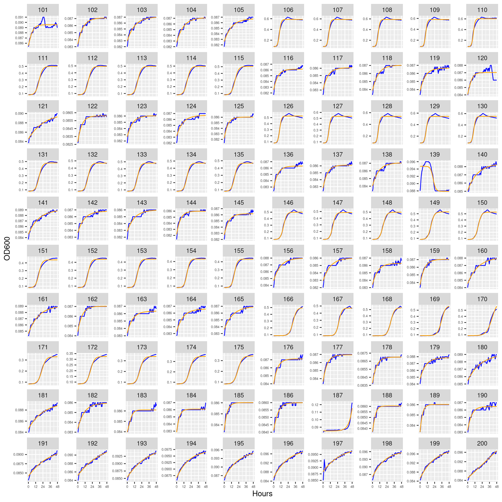
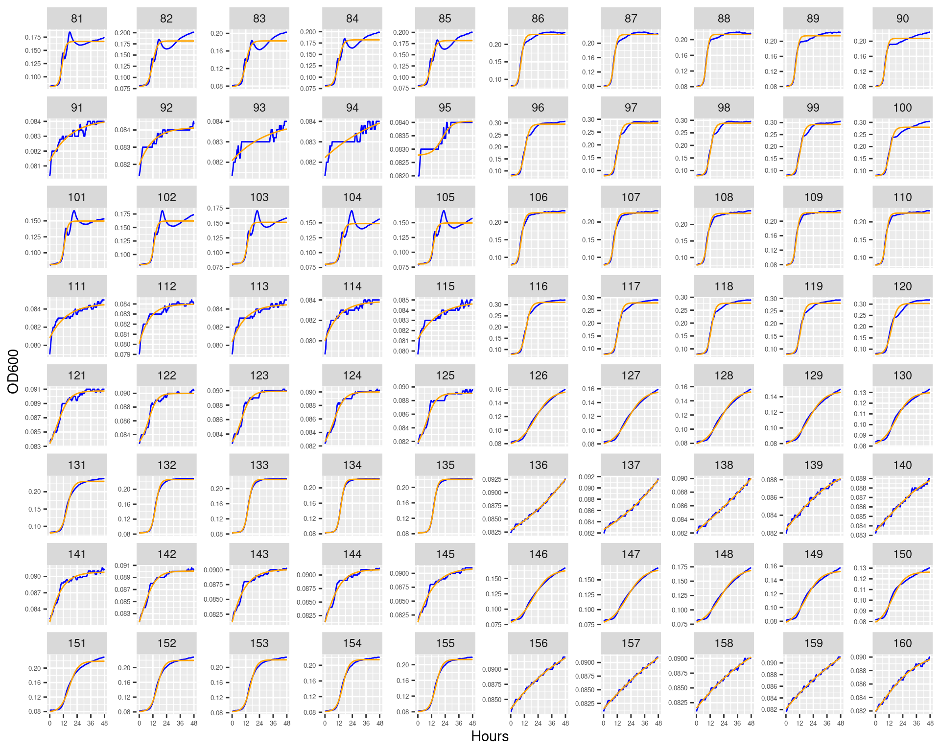
Figure 42: Bioscreen plate “bioscreen_strep_01” wells 101-200. Blue line is smoothed with a moving average window of 5 points. Orange is fitted to the Huang model.
6.4.4.2 bioscreen_strep_02
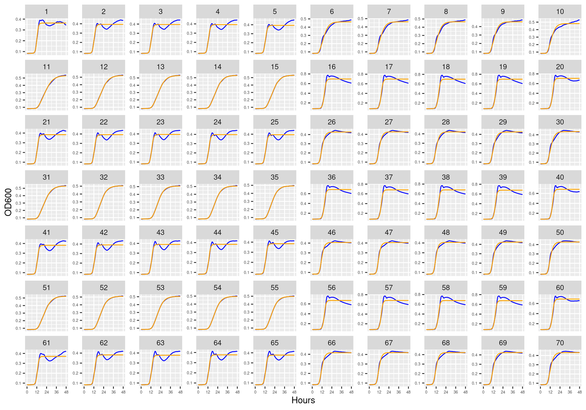
Figure 43: Bioscreen plate “bioscreen_strep_02” wells 1-70. Blue line is smoothed with a moving average window of 5 points. Orange is fitted to the Huang model.
Figure 44: Bioscreen plate “bioscreen_strep_02” wells 71-140. Blue line is smoothed with a moving average window of 5 points. Orange is fitted to the Huangv model.
6.4.4.3 bioscreen_strep_03
Figure 45: Bioscreen plate “bioscreen_strep_03” wells 1-70. Blue line is smoothed with a moving average window of 5 points. Orange is fitted to the Huang model.
Figure 46: Bioscreen plate “bioscreen_strep_03” wells 71-140. Blue line is smoothed with a moving average window of 5 points. Orange is fitted to the Huang model.
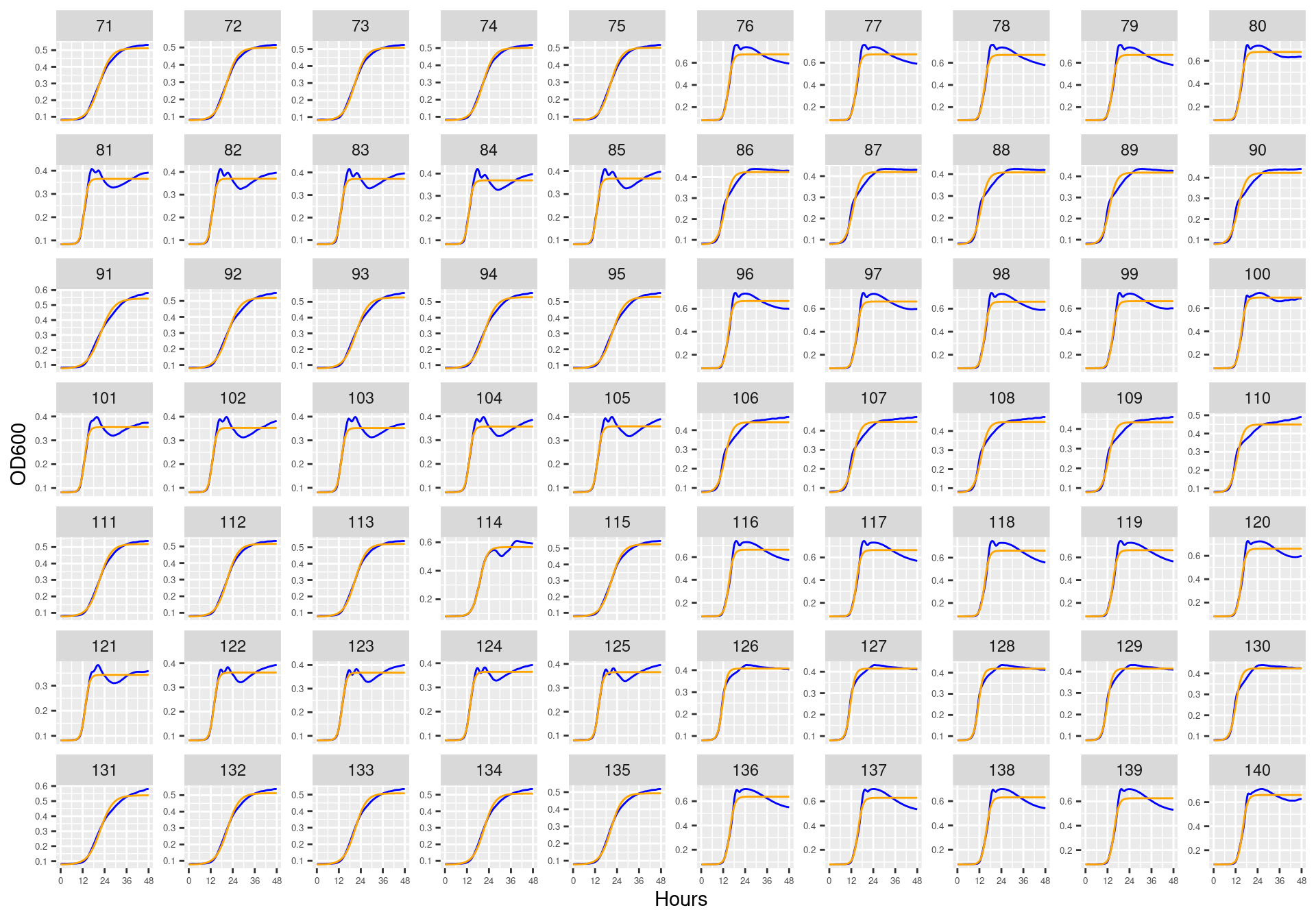
6.4.4.4 bioscreen_pairwise_filtrates_01
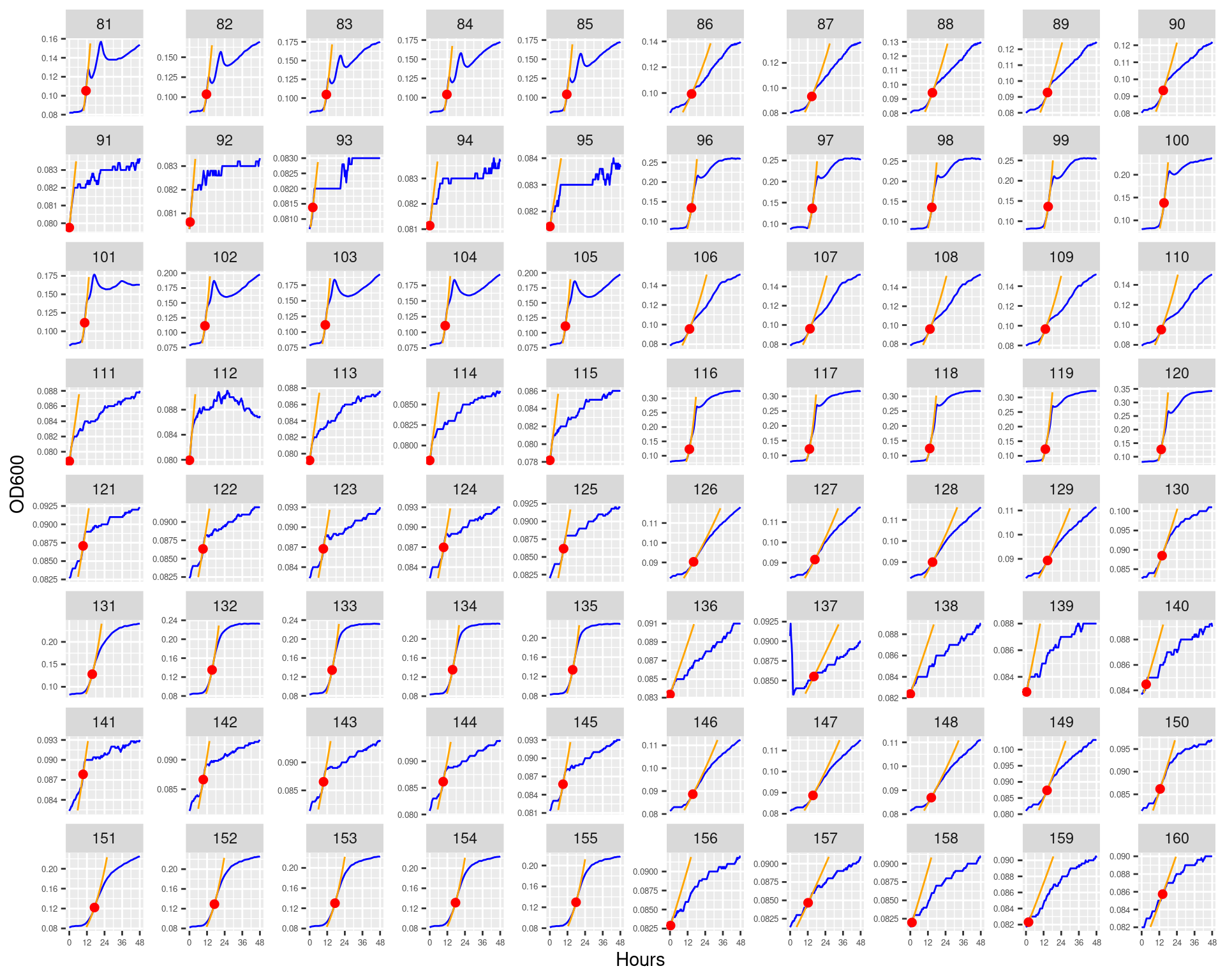
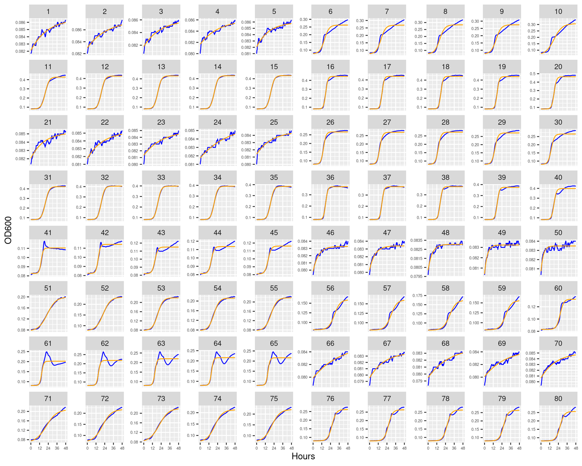
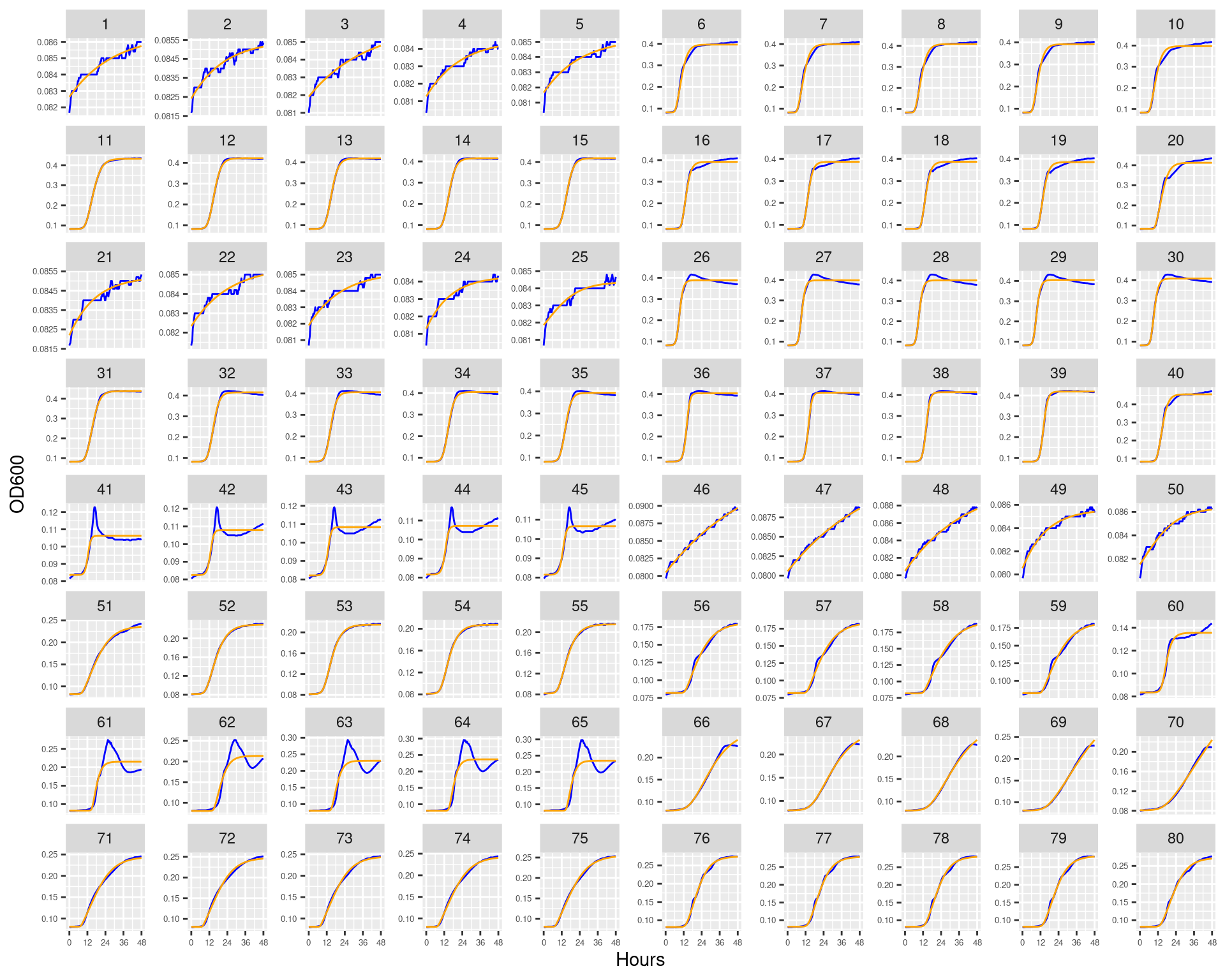
Figure 47: Bioscreen plate “bioscreen_pairwise_filtrates_01” wells 1-80. Blue line is smoothed with a moving average window of 5 points. Orange is fitted to the Huang model.
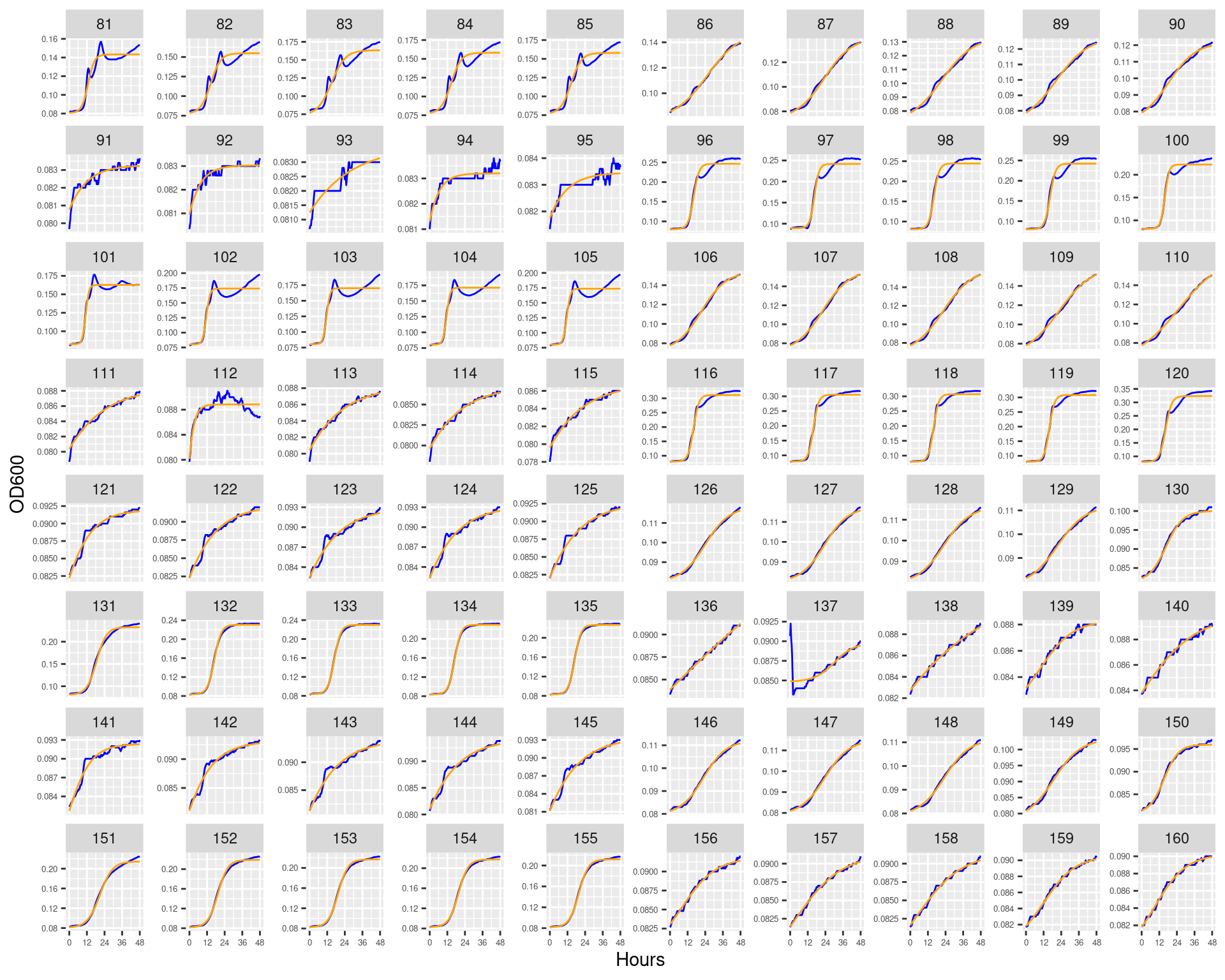
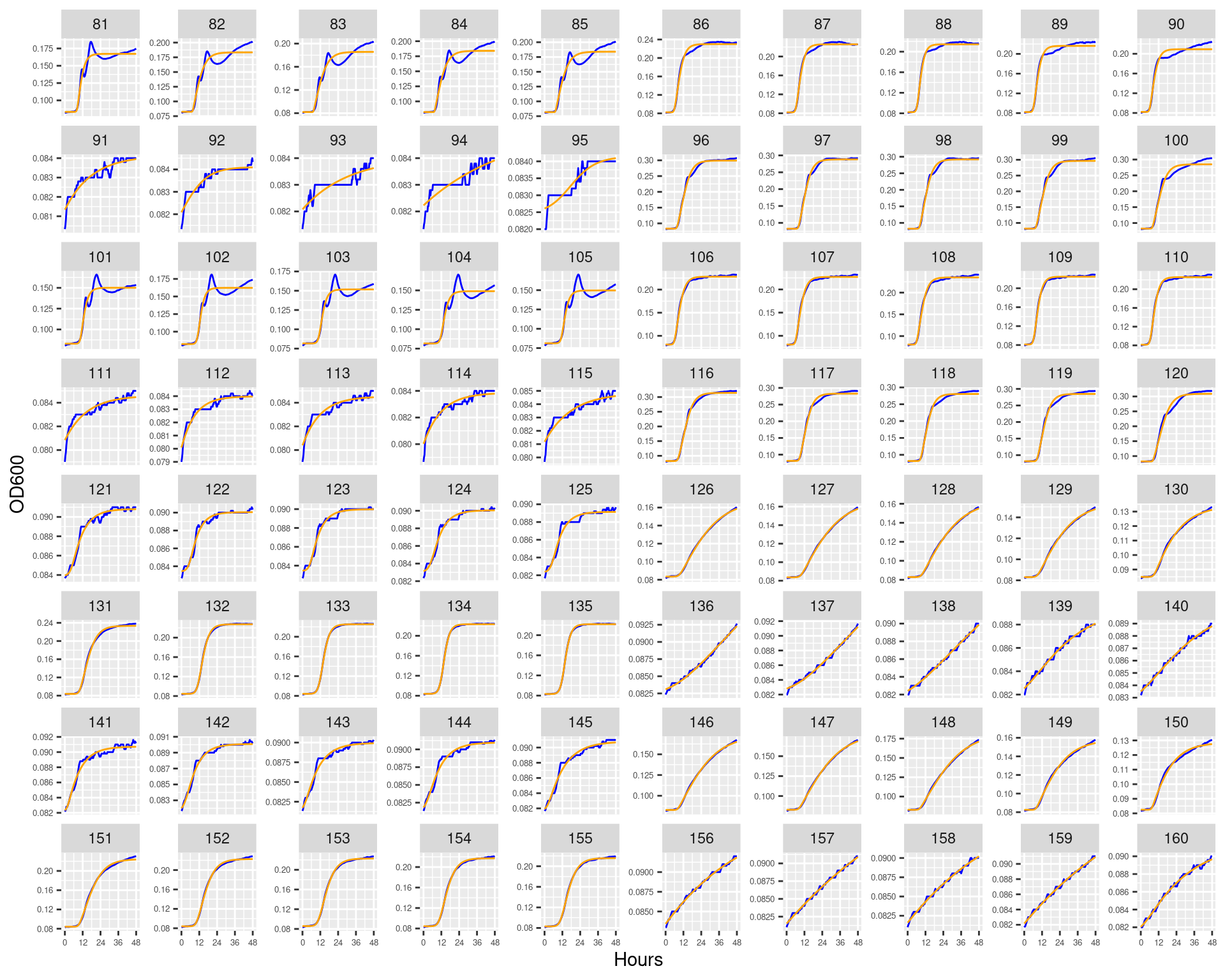
Figure 48: Bioscreen plate “bioscreen_pairwise_filtrates_01” wells 81-160. Blue line is smoothed with a moving average window of 5 points. Orange is fitted to the Huang model.
6.4.4.5 bioscreen_pairwise_filtrates_02
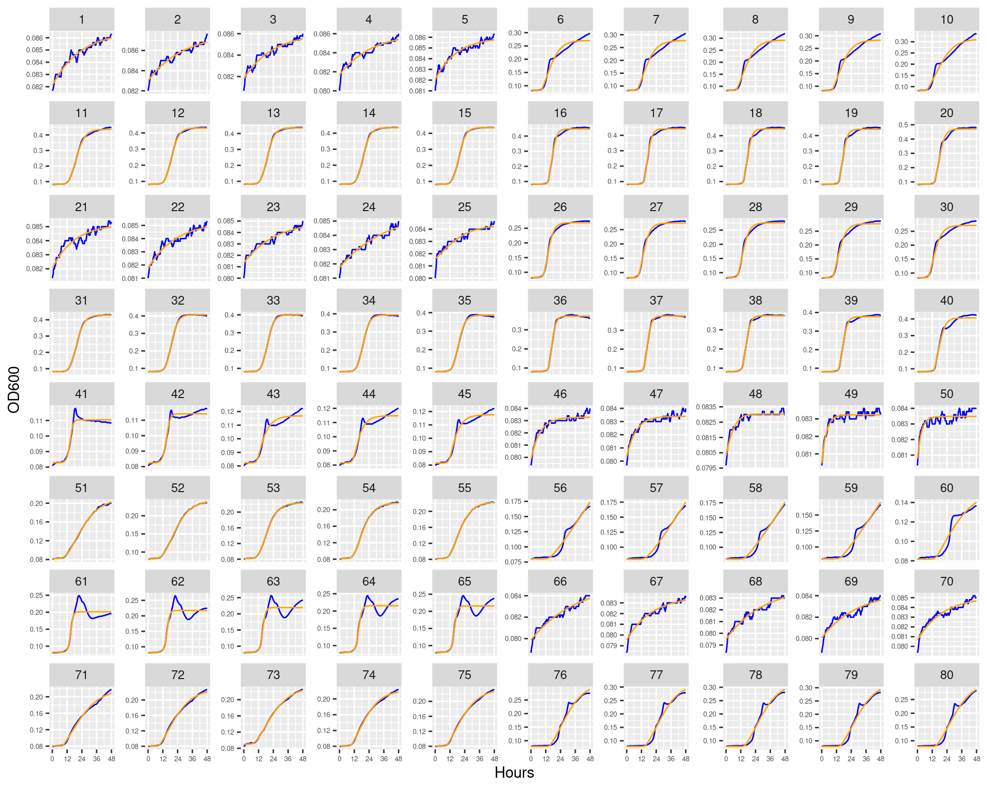
Figure 49: Bioscreen plate “bioscreen_pairwise_filtrates_02” wells 1-80. Blue line is smoothed with a moving average window of 5 points. Orange is fitted to the Huang model.
Figure 50: Bioscreen plate “bioscreen_pairwise_filtrates_02” wells 81-160. Blue line is smoothed with a moving average window of 5 points. Orange is fitted to the Huang model.
---title: "Formatting bioscreen growth curves"author: "Shane Hogle"date: todaylink-citations: true---# IntroductionBefore the main experiment we grew each ancestral and evolved form of each species in 100% R2A media at a range of streptomycin concentrations. We measured the optical density of the cultures in a high-throughput platereader [(Bioscreen)](https://www.bioscreen.fi/) over 48 hours. From this data we can estimate the growth rate and the carrying capacity of each species in the different streptomycin concentrations.We also grew all the ancestral and evolved forms of each species for 48 hours in 100% R2A media. We filtered the spent media of each species and evolved form, collected the filtrate, and grew each species/evo form in the filtrate of every other species. Again, we measured the optical density of the cultures grown on these filtrates in a high-throughput platereader [(Bioscreen)](https://www.bioscreen.fi/) over 48 hours.In this notebook we will read the output from the bioscreen plate reader and format it for later plotting and analysis.# Setup## Libraries```{r}#| output: false#| warning: false#| error: falselibrary(here)library(tidyverse)library(stringr)library(lubridate)library(fs)library(ggforce)library(slider)source(here::here("R", "utils_generic.R"))```## Global variables```{r}#| output: false#| warning: false#| error: falsedata_raw <- here::here("_data_raw", "monocultures", "20240328_bioscreen")data <- here::here("data", "monocultures", "20240328_bioscreen")# make processed data directory if it doesn't existfs::dir_create(data)```## FunctionsFor plotting results```{r}plotplate <-function(df, dfxy, unsmoothed=TRUE, predicted=FALSE, plate, rows, cols, page){ dffilt <- dplyr::filter(df, plate_name == {{ plate }}) xyfilt <-if (!is.null(dfxy)){ left_join(dfxy, distinct(dffilt, id, bioscreen_well, plate_name), by =join_by(id)) %>%drop_na()}ggplot(dffilt, aes(x = hours)) +list( ggplot2::geom_line(aes(y=OD600_rollmean), color ="blue"), if (unsmoothed) {ggplot2::geom_line(aes(y=OD600), color ="orange", lty =2)},if (predicted) {ggplot2::geom_line(aes(y=predicted), color ="orange")}, if (!is.null(dfxy)) {ggplot2::geom_point(data = xyfilt, aes(x = x, y = y), color ="red", size =2)}, ggplot2::labs(x ="Hours", y ="OD600"), ggplot2::scale_x_continuous(breaks =seq(0, 48, 12), labels =seq(0, 48, 12)), ggforce::facet_wrap_paginate(~ bioscreen_well, nrow = rows, ncol = cols, page = page, scales ="free_y"), ggplot2::theme(axis.text =element_text(size =5)) )}```# Tidying growth curves from bioscreen## Deal with encoding issuesFirst we need to know what encoding the file has```{r}readr::guess_encoding( here::here(data_raw,"bioscreen_strep_01.txt" ))```Bioscreen files are in UTF-16E.### List files```{r}files <- fs::dir_ls(path = data_raw,all =FALSE,recurse =TRUE,type ="file",glob ="*.txt",regexp =NULL,invert =FALSE,fail =TRUE)files_named <- rlang::set_names(files, nm = purrr::map_chr(files, fs::path_file) %>%str_remove(".txt"))```### Read file using base RMust use read.delim as it is the only tool that I could find that handled the UTF-16LE correctly```{r}raw_df <- purrr::map( files_named, read.delim,# this is the encoding we deduced abovefileEncoding ="UTF-16LE",skipNul =TRUE,# telling it there is no header for colulmn namesheader =FALSE,sep =" ",colClasses ="character",strip.white =TRUE,na.strings ="",# skip the first 3 lines becauseskip =3,quote ="",allowEscapes =FALSE,comment.char ="",) %>% purrr::list_rbind(names_to ="plate_name")```### Fix locale issues```{r}raw_df_decimal <- readr::type_convert( raw_df,locale = readr::locale(decimal_mark =",", grouping_mark ="."),cols(.default =col_double(),plate_name =col_character(),V1 =col_time(format =""),V203 =col_logical() )) %>% tibble::as_tibble()```### Fix weird time encodingThe `V1` variable has time encoded as `Hr:Min:Sec` which we want to convert to just secondsThe rounding step is necessary because the bioscreen actually doesn't output consistent intervals. Sometimes it is 00:30:06 and other times it is 00:30:05. This becomes a problem later on when trying to combine multiple runs at once```{r}round_any <-function(x, accuracy, f=round){f(x/ accuracy) * accuracy}raw_df_decimal_sec <- dplyr::mutate(raw_df_decimal, V1 =round_any(lubridate::period_to_seconds(lubridate::hms(V1)), 100) )```### Remove extraneous columns.Some of the columns have no useful data whatsoever. We need to get rid of those.```{r}dplyr::select(raw_df_decimal_sec, tidyselect::last_col(offset =1), tidyselect::last_col())``````{r}dplyr::select(raw_df_decimal_sec, tidyselect::num_range("V", 1:4))```The last columns is `V203` and has nothing. Column `V2` is just blank. Now we'll just keep the columns we need.```{r}gcurves_slurped_fmt <- raw_df_decimal_sec %>% dplyr::select(plate_name, V1, V3:V202) %>% dplyr::mutate(hours = lubridate::time_length(V1, unit ="hours")) %>% tidyr::pivot_longer(c(-plate_name, -hours, -V1), names_to ="well", values_to ="OD600") %>%# here we remove the V part and subtract 2 so that bioscreen well numbers will go from 1:100 per plate dplyr::mutate(bioscreen_well =as.numeric(str_remove(well, "V"))-2) %>% dplyr::rename(seconds = V1) ```# Format growth curves## Read metadataStreptomycin and filtrate conditions```{r}gcurves_slurped_fmt_md <- readr::read_tsv( here::here(data_raw, "plate_conditions.tsv"),col_names =TRUE,cols(plate_name =col_character(),plate_number =col_double(),bioscreen_well =col_double(),replicate =col_double(),sp_hist =col_character(),strep_conc =col_double(),sp_filtrate =col_character() ))```## Join with metadata to remove ununsed samples```{r}gcurves <- dplyr::left_join( gcurves_slurped_fmt_md, gcurves_slurped_fmt,by = dplyr::join_by(plate_name, bioscreen_well))```One thing I've realized is that many methods for inferring growth rates struggle when the density of observations is too high (e.g., one measurement every 5 minutes). In reality I've found that taking one measurement every 15 minutes is sufficient. Here we thin it out so that measurements are in 20 minute intervals. This seems to improve the fitting procedure a lot without much of a cost.```{r}gcurves_thin <- gcurves %>%# 1200 is 20 minutes so by ensuring modulo = 0 we include only time points# 0, 20, 40, 60 minutes and so on... dplyr::filter(seconds %%1200==0)```Now we'll do some smoothing to reduce the "jaggedness" of the curves a bit. We use the `slider` package with a 5 point rolling mean for each focal observation we take the mean including the focal point and two points before and after.```{r}gcurves_thin_sm <- gcurves_thin %>% dplyr::group_by(plate_name, bioscreen_well) %>% dplyr::mutate(OD600_rollmean = slider::slide_dbl(OD600, mean, .before =2, .after =2)) %>%ungroup()readr::write_tsv(gcurves_thin_sm, here::here(data, "gcurves_formatted_thinned.tsv"))```# Inspect growth curves## bioscreen_strep_01::: {#fig-01}```{r}#| fig.width: 10#| fig.height: 10#| echo: false#| warning: falseplotplate(gcurves_thin_sm, dfxy=NULL, unsmoothed=TRUE, predicted=FALSE, plate="bioscreen_strep_01", rows=10, cols=10, page=1)```Bioscreen plate "bioscreen_strep_01" wells 1-100. Blue line is smoothed with a moving average window of 9 points. Orange is non-smoothed:::::: {#fig-02}```{r}#| fig.width: 10#| fig.height: 10#| echo: false#| warning: falseplotplate(gcurves_thin_sm, dfxy=NULL, unsmoothed=TRUE, predicted=FALSE, plate="bioscreen_strep_01", rows=10, cols=10, page=2)```Bioscreen plate "bioscreen_strep_01" wells 101-200. Blue line is smoothed with a moving average window of 9 points. Orange is non-smoothed:::## bioscreen_strep_02::: {#fig-03}```{r}#| fig.width: 10#| fig.height: 7#| echo: false#| warning: falseplotplate(gcurves_thin_sm, dfxy=NULL, unsmoothed=TRUE, predicted=FALSE, plate="bioscreen_strep_02", rows=7, cols=10, page=1)```Bioscreen plate "bioscreen_strep_02" wells 1-70. Blue line is smoothed with a moving average window of 9 points. Orange is non-smoothed:::::: {#fig-04}```{r}#| fig.width: 10#| fig.height: 7#| echo: false#| warning: falseplotplate(gcurves_thin_sm, dfxy=NULL, unsmoothed=TRUE, predicted=FALSE, plate="bioscreen_strep_02", rows=7, cols=10, page=2)```Bioscreen plate "bioscreen_strep_02" wells 71-140. Blue line is smoothed with a moving average window of 9 points. Orange is non-smoothed:::## bioscreen_strep_03::: {#fig-05}```{r}#| fig.width: 10#| fig.height: 7#| echo: false#| warning: falseplotplate(gcurves_thin_sm, dfxy=NULL, unsmoothed=TRUE, predicted=FALSE, plate="bioscreen_strep_03", rows=7, cols=10, page=1)```Bioscreen plate "bioscreen_strep_03" wells 1-70 Blue line is smoothed with a moving average window of 9 points. Orange is non-smoothed:::::: {#fig-06}```{r}#| fig.width: 10#| fig.height: 7#| echo: false#| warning: falseplotplate(gcurves_thin_sm, dfxy=NULL, unsmoothed=TRUE, predicted=FALSE, plate="bioscreen_strep_03", rows=7, cols=10, page=2)```Bioscreen plate "bioscreen_strep_03" wells 71-140. Blue line is smoothed with a moving average window of 9 points. Orange is non-smoothed:::## bioscreen_pairwise_filtrates_01::: {#fig-07}```{r}#| fig.width: 10#| fig.height: 8#| echo: false#| warning: falseplotplate(gcurves_thin_sm, dfxy=NULL, unsmoothed=TRUE, predicted=FALSE, plate="bioscreen_pairwise_filtrates_01", rows=8, cols=10, page=1)```Bioscreen plate "bioscreen_pairwise_filtrates_01" wells 1-80 Blue line is smoothed with a moving average window of 9 points. Orange is non-smoothed:::::: {#fig-08}```{r}#| fig.width: 10#| fig.height: 8#| echo: false#| warning: falseplotplate(gcurves_thin_sm, dfxy=NULL, unsmoothed=TRUE, predicted=FALSE, plate="bioscreen_pairwise_filtrates_01", rows=8, cols=10, page=2)```Bioscreen plate "bioscreen_pairwise_filtrates_01" wells 81-160 Blue line is smoothed with a moving average window of 9 points. Orange is non-smoothed:::## bioscreen_pairwise_filtrates_02::: {#fig-09}```{r}#| fig.width: 10#| fig.height: 8#| echo: false#| warning: falseplotplate(gcurves_thin_sm, dfxy=NULL, unsmoothed=TRUE, predicted=FALSE, plate="bioscreen_pairwise_filtrates_02", rows=8, cols=10, page=1)```Bioscreen plate "bioscreen_pairwise_filtrates_02" wells 1-80. Blue line is smoothed with a moving average window of 9 points. Orange is non-smoothed:::::: {#fig-10}```{r}#| fig.width: 10#| fig.height: 8#| echo: false#| warning: falseplotplate(gcurves_thin_sm, dfxy=NULL, unsmoothed=TRUE, predicted=FALSE, plate="bioscreen_pairwise_filtrates_02", rows=8, cols=10, page=2)```Bioscreen plate "bioscreen_pairwise_filtrates_02" wells 81-160. Blue line is smoothed with a moving average window of 9 points. Orange is non-smoothed:::## ConclusionsGrowth curves all look reasonable. Can proceed with the analysis.# Growth curve statistics```{r}library("growthrates")library("DescTools")```Using the tool [`growthrates`](https://cran.r-project.org/web/packages/growthrates/index.html) to estimate mu_max. I have found this works a lot better the gcplyr and is more convenient than using another tool outside of R. Nonparametric estimate growth rates by spline is very fast. Fitting to a model takes more time resources. [Generally it is best to try multiple approaches and to visualize/check the data to make sure it makes sense.](https://www.frontiersin.org/journals/ecology-and-evolution/articles/10.3389/fevo.2023.1313500/full)```{r}gcurves_thin_sm <- gcurves_thin_sm %>%# make uniq idmutate(id =paste0(plate_name, "|", bioscreen_well))```## Spline based estiamteSmoothing splines are a quick method to estimate maximum growth. The method is called nonparametric, because the growth rate is directly estimated from the smoothed data without being restricted to a specific model formula.From [growthrates documentation:](https://cran.r-project.org/web/packages/growthrates/growthrates.pdf)> The method was inspired by an algorithm of [Kahm et al. (2010)](https://www.jstatsoft.org/article/view/v033i07), with different settings and assumptions. In the moment, spline fitting is always done with log-transformed data, assuming exponential growth at the time point of the maximum of the first derivative of the spline fit. All the hard work is done by function smooth.spline from package stats, that is highly user configurable. Normally, smoothness is automatically determined via cross-validation. This works well in many cases, whereas manual adjustment is required otherwise, e.g. by setting spar to a fixed value \[0, 1\] that also disables cross-validation.### Fit```{r}#| eval: falseset.seed(45278)many_spline <- growthrates::all_splines(OD600_rollmean ~ hours | id, data = gcurves_thin_sm, spar =0.5)readr::write_rds(many_spline, here::here(data, "spline_fits"))``````{r}#| echo: false#| warning: falsemany_spline <- readr::read_rds(here::here(data, "spline_fits"))```### Results```{r}many_spline_res <- growthrates::results(many_spline)```### Predictions```{r}many_spline_xy <- purrr::map(many_spline@fits, \(x) data.frame(x = x@xy[1], y = x@xy[2])) %>% purrr::list_rbind(names_to ="id") %>% dplyr::mutate(id = stringr::str_remove_all(id, "bioscreen_pairwise_|bioscreen_"))many_spline_fitted <- purrr::map(many_spline@fits, \(x) data.frame(x@FUN(x@obs$time, x@par))) %>% purrr::list_rbind(names_to ="id") %>% dplyr::rename(hours = time, predicted = y) %>% dplyr::left_join(gcurves_thin_sm, by = dplyr::join_by(id, hours)) %>% dplyr::mutate(id = stringr::str_remove_all(id, "bioscreen_pairwise_|bioscreen_")) %>% dplyr::group_by(id) %>%# this step makes sure we don't plot fits that go outside the range of the data dplyr::mutate(predicted = dplyr::if_else(dplyr::between(predicted, min(OD600_rollmean), max(OD600_rollmean)), predicted, NA_real_)) %>% dplyr::ungroup()```### Plot#### bioscreen_strep_01::: {#fig-11}```{r}#| fig.width: 10#| fig.height: 10#| echo: false#| warning: falseplotplate(many_spline_fitted, dfxy=many_spline_xy, unsmoothed=FALSE, predicted=TRUE, plate="bioscreen_strep_01", rows=10, cols=10, page=1)```Bioscreen plate "bioscreen_strep_01" wells 1-100. Blue line is smoothed with a moving average window of 5 points. Orange is slope of max predicted growth rate from the first derivative of a smoothing spline. Red dot is hours and OD600 at which maximum growth rate is reached.:::::: {#fig-12}```{r}#| fig.width: 10#| fig.height: 10#| echo: false#| warning: falseplotplate(many_spline_fitted, dfxy=many_spline_xy, unsmoothed=FALSE, predicted=TRUE, plate="bioscreen_strep_01", rows=10, cols=10, page=2)```Bioscreen plate "bioscreen_strep_01" wells 101-200. Blue line is smoothed with a moving average window of 5 points. Orange is slope of max predicted growth rate from the first derivative of a smoothing spline. Red dot is hours and OD600 at which maximum growth rate is reached.:::#### bioscreen_strep_02::: {#fig-13}```{r}#| fig.width: 10#| fig.height: 7#| echo: false#| warning: falseplotplate(many_spline_fitted, dfxy=many_spline_xy, unsmoothed=FALSE, predicted=TRUE, plate="bioscreen_strep_02", rows=7, cols=10, page=1)```Bioscreen plate "bioscreen_strep_02" wells 1-70. Blue line is smoothed with a moving average window of 5 points. Orange is slope of max predicted growth rate from the first derivative of a smoothing spline. Red dot is hours and OD600 at which maximum growth rate is reached.:::::: {#fig-14}```{r}#| fig.width: 10#| fig.height: 7#| echo: false#| warning: falseplotplate(many_spline_fitted, dfxy=many_spline_xy, unsmoothed=FALSE, predicted=TRUE, plate="bioscreen_strep_02", rows=7, cols=10, page=2)```Bioscreen plate "bioscreen_strep_02" wells 71-140. Blue line is smoothed with a moving average window of 5 points. Orange is slope of max predicted growth rate from the first derivative of a smoothing spline. Red dot is hours and OD600 at which maximum growth rate is reached.:::#### bioscreen_strep_03::: {#fig-15}```{r}#| fig.width: 10#| fig.height: 7#| echo: false#| warning: falseplotplate(many_spline_fitted, dfxy=many_spline_xy, unsmoothed=FALSE, predicted=TRUE, plate="bioscreen_strep_03", rows=7, cols=10, page=1)```Bioscreen plate "bioscreen_strep_03" wells 1-70. Blue line is smoothed with a moving average window of 5 points. Orange is slope of max predicted growth rate from the first derivative of a smoothing spline. Red dot is hours and OD600 at which maximum growth rate is reached.:::::: {#fig-16}```{r}#| fig.width: 10#| fig.height: 7#| echo: false#| warning: falseplotplate(many_spline_fitted, dfxy=many_spline_xy, unsmoothed=FALSE, predicted=TRUE, plate="bioscreen_strep_03", rows=7, cols=10, page=2)```Bioscreen plate "bioscreen_strep_03" wells 71-140. Blue line is smoothed with a moving average window of 5 points. Orange is slope of max predicted growth rate from the first derivative of a smoothing spline. Red dot is hours and OD600 at which maximum growth rate is reached.:::#### bioscreen_pairwise_filtrates_01::: {#fig-17}```{r}#| fig.width: 10#| fig.height: 8#| echo: false#| warning: falseplotplate(many_spline_fitted, dfxy=many_spline_xy, unsmoothed=FALSE, predicted=TRUE, plate="bioscreen_pairwise_filtrates_01", rows=8, cols=10, page=1)```Bioscreen plate "bioscreen_pairwise_filtrates_01" wells 1-80. Blue line is smoothed with a moving average window of 5 points. Orange is slope of max predicted growth rate. Red dot is hours and OD600 at which maximum growth rate is reached.:::::: {#fig-18}```{r}#| fig.width: 10#| fig.height: 8#| echo: false#| warning: falseplotplate(many_spline_fitted, dfxy=many_spline_xy, unsmoothed=FALSE, predicted=TRUE, plate="bioscreen_pairwise_filtrates_01", rows=8, cols=10, page=2)```Bioscreen plate "bioscreen_pairwise_filtrates_01" wells 81-160. Blue line is smoothed with a moving average window of 5 points. Orange is slope of max predicted growth rate. Red dot is hours and OD600 at which maximum growth rate is reached.:::#### bioscreen_pairwise_filtrates_02::: {#fig-19}```{r}#| fig.width: 10#| fig.height: 8#| echo: false#| warning: falseplotplate(many_spline_fitted, dfxy=many_spline_xy, unsmoothed=FALSE, predicted=TRUE, plate="bioscreen_pairwise_filtrates_02", rows=8, cols=10, page=1)```Bioscreen plate "bioscreen_pairwise_filtrates_02" wells 1-80. Blue line is smoothed with a moving average window of 5 points. Orange is slope of max predicted growth rate. Red dot is hours and OD600 at which maximum growth rate is reached.:::::: {#fig-20}```{r}#| fig.width: 10#| fig.height: 8#| echo: false#| warning: falseplotplate(many_spline_fitted, dfxy=many_spline_xy, unsmoothed=FALSE, predicted=TRUE, plate="bioscreen_pairwise_filtrates_02", rows=8, cols=10, page=2)```Bioscreen plate "bioscreen_pairwise_filtrates_02" wells 81-160. Blue line is smoothed with a moving average window of 5 points. Orange is slope of max predicted growth rate. Red dot is hours and OD600 at which maximum growth rate is reached.:::## Linear model based estimateThis method determine maximum growth rates from the log-linear part of a growth curve using a heuristic approach similar to the "growth rates made easy" method of [Hall et al. (2013).](https://doi.org/10.1093/molbev/mst187)From [growthrates documentation:](https://cran.r-project.org/web/packages/growthrates/growthrates.pdf)> The algorithm works as follows:>> 1\. Fit linear regressions to all subsets of h consecutive data points. If for example h = 5, fit a linear regression to points 1 . . . 5, 2 . . . 6, 3. . . 7 and so on. The method seeks the highest rate of exponential growth, so the dependent variable is of course log-transformed.>> 2\. Find the subset with the highest slope bmax and include also the data points of adjacent subsets that have a slope of at least quota · bmax, e.g. all data sets that have at least 95% of the maximum slope.>> 3\. Fit a new linear model to the extended data window identified in step 2.### Fit```{r}#| eval: falseset.seed(45278)many_linear <- growthrates::all_easylinear(OD600_rollmean ~ hours | id, data = gcurves_thin_sm)readr::write_rds(many_linear, here::here(data, "linear_fits"))``````{r}#| echo: false#| warning: falsemany_linear <- readr::read_rds(here::here(data, "linear_fits"))```### Results```{r}many_linear_res <- growthrates::results(many_linear)```### Predictions```{r}many_linear_fitted <- purrr::map(many_spline@fits, \(x) data.frame(x@FUN(x@obs$time, x@par))) %>% purrr::list_rbind(names_to ="id") %>% dplyr::rename(hours = time, predicted = y) %>% dplyr::left_join(gcurves_thin_sm, by = dplyr::join_by(id, hours)) %>% dplyr::mutate(id = stringr::str_remove_all(id, "bioscreen_pairwise_|bioscreen_")) %>% dplyr::group_by(id) %>%# this step makes sure we don't plot fits that go outside the range of the data dplyr::mutate(predicted = dplyr::if_else(dplyr::between(predicted, min(OD600_rollmean), max(OD600_rollmean)), predicted, NA_real_)) %>% dplyr::ungroup()```### Plot#### bioscreen_strep_01::: {#fig-21}```{r}#| fig.width: 10#| fig.height: 10#| echo: false#| warning: falseplotplate(many_linear_fitted, dfxy=NULL, unsmoothed=FALSE, predicted=TRUE, plate="bioscreen_strep_01", rows=10, cols=10, page=1)```Bioscreen plate "bioscreen_strep_01" wells 1-100. Blue line is smoothed with a moving average window of 5 points. Orange is slope of max predicted growth rate from a piecewise linear model fit.:::::: {#fig-22}```{r}#| fig.width: 10#| fig.height: 10#| echo: false#| warning: falseplotplate(many_linear_fitted, dfxy=NULL, unsmoothed=FALSE, predicted=TRUE, plate="bioscreen_strep_01", rows=10, cols=10, page=2)```Bioscreen plate "bioscreen_strep_01" wells 101-200. Blue line is smoothed with a moving average window of 5 points. Orange is slope of max predicted growth rate from a piecewise linear model fit.:::#### bioscreen_strep_02::: {#fig-23}```{r}#| fig.width: 10#| fig.height: 7#| echo: false#| warning: falseplotplate(many_linear_fitted, dfxy=NULL, unsmoothed=FALSE, predicted=TRUE, plate="bioscreen_strep_02", rows=7, cols=10, page=1)```Bioscreen plate "bioscreen_strep_02" wells 1-70. Blue line is smoothed with a moving average window of 5 points. Orange is slope of max predicted growth rate from a piecewise linear model fit.:::::: {#fig-24}```{r}#| fig.width: 10#| fig.height: 7#| echo: false#| warning: falseplotplate(many_linear_fitted, dfxy=NULL, unsmoothed=FALSE, predicted=TRUE, plate="bioscreen_strep_02", rows=7, cols=10, page=2)```Bioscreen plate "bioscreen_strep_02" wells 71-140. Blue line is smoothed with a moving average window of 5 points. Orange is slope of max predicted growth rate from a piecewise linear model fit.:::#### bioscreen_strep_03::: {#fig-25}```{r}#| fig.width: 10#| fig.height: 7#| echo: false#| warning: falseplotplate(many_linear_fitted, dfxy=NULL, unsmoothed=FALSE, predicted=TRUE, plate="bioscreen_strep_03", rows=7, cols=10, page=1)```Bioscreen plate "bioscreen_strep_03" wells 1-70. Blue line is smoothed with a moving average window of 5 points. Orange is slope of max predicted growth rate from a piecewise linear model fit.:::::: {#fig-26}```{r}#| fig.width: 10#| fig.height: 7#| echo: false#| warning: falseplotplate(many_linear_fitted, dfxy=NULL, unsmoothed=FALSE, predicted=TRUE, plate="bioscreen_strep_03", rows=7, cols=10, page=2)```Bioscreen plate "bioscreen_strep_03" wells 71-140. Blue line is smoothed with a moving average window of 5 points. Orange is slope of max predicted growth rate from a piecewise linear model fit.:::#### bioscreen_pairwise_filtrates_01::: {#fig-27}```{r}#| fig.width: 10#| fig.height: 8#| echo: false#| warning: falseplotplate(many_linear_fitted, dfxy=NULL, unsmoothed=FALSE, predicted=TRUE, plate="bioscreen_pairwise_filtrates_01", rows=8, cols=10, page=1)```Bioscreen plate "bioscreen_pairwise_filtrates_01" wells 1-80. Blue line is smoothed with a moving average window of 5 points. Orange is slope of max predicted growth rate from a piecewise linear model fit.:::::: {#fig-28}```{r}#| fig.width: 10#| fig.height: 8#| echo: false#| warning: falseplotplate(many_linear_fitted, dfxy=NULL, unsmoothed=FALSE, predicted=TRUE, plate="bioscreen_pairwise_filtrates_01", rows=8, cols=10, page=2)```Bioscreen plate "bioscreen_pairwise_filtrates_01" wells 81-160. Blue line is smoothed with a moving average window of 5 points. Orange is slope of max predicted growth rate from a piecewise linear model fit.:::#### bioscreen_pairwise_filtrates_02::: {#fig-29}```{r}#| fig.width: 10#| fig.height: 8#| echo: false#| warning: falseplotplate(many_linear_fitted, dfxy=NULL, unsmoothed=FALSE, predicted=TRUE, plate="bioscreen_pairwise_filtrates_02", rows=8, cols=10, page=1)```Bioscreen plate "bioscreen_pairwise_filtrates_02" wells 1-80. Blue line is smoothed with a moving average window of 5 points. Orange is slope of max predicted growth rate from a piecewise linear model fit.:::::: {#fig-30}```{r}#| fig.width: 10#| fig.height: 8#| echo: false#| warning: falseplotplate(many_linear_fitted, dfxy=NULL, unsmoothed=FALSE, predicted=TRUE, plate="bioscreen_pairwise_filtrates_02", rows=8, cols=10, page=2)```Bioscreen plate "bioscreen_pairwise_filtrates_02" wells 81-160. Blue line is smoothed with a moving average window of 5 points. Orange is slope of max predicted growth rate from a piecewise linear model fit.:::## Baranyi parametric fit estimateThis uses the growth model of [Baranyi and Roberts (1995)](https://www.sciencedirect.com/science/article/pii/016816059400121L) written as analytical solution of the system of differential equations.From [growthrates documentation:](https://cran.r-project.org/web/packages/growthrates/growthrates.pdf)> The version of the equation used in this package has the following form:>> $A = time + \frac{1}{mumax} \times \log((−\mu_{max} \times time) +exp(−h_{0})−exp(−\mu_{max} \times time−h0))$>> $\log(y) = \log(y_{0}) + \mu_{max} \times A − log(1 + \frac{\exp(\mu_{max} \times A) − 1}{\exp(\log(K) − \log(y_{0})})$### Fit```{r}#| eval: falseset.seed(783622)# starting values and limits for the baranyi modelp <-c(y0 =0.03, mumax = .1, K =0.1, h0 =1)lower <-c(y0 =0.001, mumax =1e-2, K =0.005, h0 =0)upper <-c(y0 =0.1, mumax =1, K =0.9, h0 =10)many_baranyi <- growthrates::all_growthmodels( OD600_rollmean ~ growthrates::grow_baranyi(hours, parms) | id,data = gcurves_thin_sm,p = p, lower = lower, upper = upper,transform ="log", ncores =8)readr::write_rds(many_baranyi, here::here(data, "barayani_fits"))``````{r}#| echo: false#| warning: falsemany_baranyi <- readr::read_rds(here::here(data, "barayani_fits"))```### Results```{r}many_baranyi_res <- growthrates::results(many_baranyi)```### Predictions```{r}many_baranyi_fitted <- purrr::map(many_baranyi@fits, \(x) data.frame(x@FUN(x@obs$time, x@par))) %>% purrr::list_rbind(names_to ="id") %>% dplyr::rename(hours = time, predicted = y) %>% dplyr::left_join(gcurves_thin_sm, by = dplyr::join_by(id, hours)) %>% dplyr::mutate(id = stringr::str_remove_all(id, "bioscreen_pairwise_|bioscreen_"))```### Plot#### bioscreen_strep_01::: {#fig-31}```{r}#| fig.width: 10#| fig.height: 10#| echo: false#| warning: falseplotplate(many_baranyi_fitted, dfxy=NULL, unsmoothed=FALSE, predicted=TRUE, plate="bioscreen_strep_01", rows=10, cols=10, page=1)```Bioscreen plate "bioscreen_strep_01" wells 1-100. Blue line is smoothed with a moving average window of 5 points. Orange is fitted to the Baranyi 1995 model.:::::: {#fig-32}```{r}#| fig.width: 10#| fig.height: 10#| echo: false#| warning: falseplotplate(many_baranyi_fitted, dfxy=NULL, unsmoothed=FALSE, predicted=TRUE, plate="bioscreen_strep_01", rows=10, cols=10, page=2)```Bioscreen plate "bioscreen_strep_01" wells 101-200. Blue line is smoothed with a moving average window of 5 points. Orange is fitted to the Baranyi 1995 model.:::#### bioscreen_strep_02::: {#fig-33}```{r}#| fig.width: 10#| fig.height: 7#| echo: false#| warning: falseplotplate(many_baranyi_fitted, dfxy=NULL, unsmoothed=FALSE, predicted=TRUE, plate="bioscreen_strep_02", rows=7, cols=10, page=1)```Bioscreen plate "bioscreen_strep_02" wells 1-70. Blue line is smoothed with a moving average window of 5 points. Orange is fitted to the Baranyi 1995 model.:::::: {#fig-34}```{r}#| fig.width: 10#| fig.height: 7#| echo: false#| warning: falseplotplate(many_baranyi_fitted, dfxy=NULL, unsmoothed=FALSE, predicted=TRUE, plate="bioscreen_strep_02", rows=7, cols=10, page=2)```Bioscreen plate "bioscreen_strep_02" wells 71-140. Blue line is smoothed with a moving average window of 5 points. Orange is fitted to the Baranyi 1995 model.:::#### bioscreen_strep_03::: {#fig-35}```{r}#| fig.width: 10#| fig.height: 7#| echo: false#| warning: falseplotplate(many_baranyi_fitted, dfxy=NULL, unsmoothed=FALSE, predicted=TRUE, plate="bioscreen_strep_03", rows=7, cols=10, page=1)```Bioscreen plate "bioscreen_strep_03" wells 1-70. Blue line is smoothed with a moving average window of 5 points. Orange is fitted to the Baranyi 1995 model.:::::: {#fig-36}```{r}#| fig.width: 10#| fig.height: 7#| echo: false#| warning: falseplotplate(many_baranyi_fitted, dfxy=NULL, unsmoothed=FALSE, predicted=TRUE, plate="bioscreen_strep_03", rows=7, cols=10, page=2)```Bioscreen plate "bioscreen_strep_03" wells 71-140. Blue line is smoothed with a moving average window of 5 points. Orange is fitted to the Baranyi 1995 model.:::#### bioscreen_pairwise_filtrates_01::: {#fig-37}```{r}#| fig.width: 10#| fig.height: 8#| echo: false#| warning: falseplotplate(many_baranyi_fitted, dfxy=NULL, unsmoothed=FALSE, predicted=TRUE, plate="bioscreen_pairwise_filtrates_01", rows=8, cols=10, page=1)```Bioscreen plate "bioscreen_pairwise_filtrates_01" wells 1-80. Blue line is smoothed with a moving average window of 5 points. Orange is fitted to the Baranyi 1995 model.:::::: {#fig-38}```{r}#| fig.width: 10#| fig.height: 8#| echo: false#| warning: falseplotplate(many_baranyi_fitted, dfxy=NULL, unsmoothed=FALSE, predicted=TRUE, plate="bioscreen_pairwise_filtrates_01", rows=8, cols=10, page=2)```Bioscreen plate "bioscreen_pairwise_filtrates_01" wells 81-160. Blue line is smoothed with a moving average window of 5 points. Orange is fitted to the Baranyi 1995 model.:::#### bioscreen_pairwise_filtrates_02::: {#fig-39}```{r}#| fig.width: 10#| fig.height: 8#| echo: false#| warning: falseplotplate(many_baranyi_fitted, dfxy=NULL, unsmoothed=FALSE, predicted=TRUE, plate="bioscreen_pairwise_filtrates_02", rows=8, cols=10, page=1)```Bioscreen plate "bioscreen_pairwise_filtrates_02" wells 1-80. Blue line is smoothed with a moving average window of 5 points. Orange is fitted to the Baranyi 1995 model.:::::: {#fig-40}```{r}#| fig.width: 10#| fig.height: 8#| echo: false#| warning: falseplotplate(many_baranyi_fitted, dfxy=NULL, unsmoothed=FALSE, predicted=TRUE, plate="bioscreen_pairwise_filtrates_02", rows=8, cols=10, page=2)```Bioscreen plate "bioscreen_pairwise_filtrates_02" wells 81-160. Blue line is smoothed with a moving average window of 5 points. Orange is fitted to the Baranyi 1995 model.:::## Huang parametric fit estimateHuangs growth model ([ref 1](https://doi.org/10.1111/j.1750-3841.2008.00785.x), [ref 2](https://doi.org/10.1016/j.fm.2010.05.019)) written as analytical solution of the differential equations.From [growthrates documentation:](https://cran.r-project.org/web/packages/growthrates/growthrates.pdf)> The version of the equation used in this package has the following form:>> $B = time + \frac{1}{alpha} \times \log(\frac{1 + exp(−\alpha \times (time - \lambda))}{1 + exp(\alpha \times \lambda})$>> $\log(y) = \log(y_{0}) + \log(K) − \log(y_{0} + (K − y_{0}) \times exp(−\mu_{max} \times B))$>> In contrast to the original publication, all parameters related to population abundance (y, y0, K) are given as untransformed values. They are not log-transformed. In general, using log-transformed parameters would indeed be a good idea to avoid the need of constained optimization, but tests showed that box-constrained optimization worked resonably well. Therefore, handling of optionally log-transformed parameters was removed from the package to avoid confusion. If you want to discuss this, please let me know.### Fit```{r}#| eval: falseset.seed(123784)# starting values and limits for the huang modelp <-c(y0 =0.03, mumax = .1, K =0.1, alpha =1.5, lambda =3)lower <-c(y0 =0.001, mumax =1e-2, K =0.005, alpha =0.1, lambda =0.03)upper <-c(y0 =0.1, mumax =1, K =0.9, alpha =15, lambda =15)many_huang <- growthrates::all_growthmodels( OD600_rollmean ~ growthrates::grow_huang(hours, parms) | id,data = gcurves_thin_sm,p = p, lower = lower, upper = upper,transform ="log", ncores =8)readr::write_rds(many_huang, here::here(data, "huang_fits"))``````{r}#| echo: false#| warning: falsemany_huang <- readr::read_rds(here::here(data, "huang_fits"))```### Results```{r}many_huang_res <- growthrates::results(many_huang)```### Predictions```{r}many_huang_fitted <- purrr::map(many_huang@fits, \(x) data.frame(x@FUN(x@obs$time, x@par))) %>% purrr::list_rbind(names_to ="id") %>% dplyr::rename(hours = time, predicted = y) %>% dplyr::left_join(gcurves_thin_sm, by = dplyr::join_by(id, hours)) %>% dplyr::mutate(id = stringr::str_remove_all(id, "bioscreen_pairwise_|bioscreen_"))```### Plot#### bioscreen_strep_01::: {#fig-41}```{r}#| fig.width: 10#| fig.height: 10#| echo: false#| warning: falseplotplate(many_huang_fitted, dfxy=NULL, unsmoothed=FALSE, predicted=TRUE, plate="bioscreen_strep_01", rows=10, cols=10, page=1)```Bioscreen plate "bioscreen_strep_01" wells 1-100. Blue line is smoothed with a moving average window of 5 points. Orange is fitted to the Huang model.:::::: {#fig-42}```{r}#| fig.width: 10#| fig.height: 10#| echo: false#| warning: falseplotplate(many_huang_fitted, dfxy=NULL, unsmoothed=FALSE, predicted=TRUE, plate="bioscreen_strep_01", rows=10, cols=10, page=2)```Bioscreen plate "bioscreen_strep_01" wells 101-200. Blue line is smoothed with a moving average window of 5 points. Orange is fitted to the Huang model.:::#### bioscreen_strep_02::: {#fig-43}```{r}#| fig.width: 10#| fig.height: 7#| echo: false#| warning: falseplotplate(many_huang_fitted, dfxy=NULL, unsmoothed=FALSE, predicted=TRUE, plate="bioscreen_strep_02", rows=7, cols=10, page=1)```Bioscreen plate "bioscreen_strep_02" wells 1-70. Blue line is smoothed with a moving average window of 5 points. Orange is fitted to the Huang model.:::::: {#fig-44}```{r}#| fig.width: 10#| fig.height: 7#| echo: false#| warning: falseplotplate(many_huang_fitted, dfxy=NULL, unsmoothed=FALSE, predicted=TRUE, plate="bioscreen_strep_02", rows=7, cols=10, page=2)```Bioscreen plate "bioscreen_strep_02" wells 71-140. Blue line is smoothed with a moving average window of 5 points. Orange is fitted to the Huangv model.:::#### bioscreen_strep_03::: {#fig-45}```{r}#| fig.width: 10#| fig.height: 7#| echo: false#| warning: falseplotplate(many_huang_fitted, dfxy=NULL, unsmoothed=FALSE, predicted=TRUE, plate="bioscreen_strep_03", rows=7, cols=10, page=1)```Bioscreen plate "bioscreen_strep_03" wells 1-70. Blue line is smoothed with a moving average window of 5 points. Orange is fitted to the Huang model.:::::: {#fig-46}```{r}#| fig.width: 10#| fig.height: 7#| echo: false#| warning: falseplotplate(many_huang_fitted, dfxy=NULL, unsmoothed=FALSE, predicted=TRUE, plate="bioscreen_strep_03", rows=7, cols=10, page=2)```Bioscreen plate "bioscreen_strep_03" wells 71-140. Blue line is smoothed with a moving average window of 5 points. Orange is fitted to the Huang model.:::#### bioscreen_pairwise_filtrates_01::: {#fig-47}```{r}#| fig.width: 10#| fig.height: 8#| echo: false#| warning: falseplotplate(many_huang_fitted, dfxy=NULL, unsmoothed=FALSE, predicted=TRUE, plate="bioscreen_pairwise_filtrates_01", rows=8, cols=10, page=1)```Bioscreen plate "bioscreen_pairwise_filtrates_01" wells 1-80. Blue line is smoothed with a moving average window of 5 points. Orange is fitted to the Huang model.:::::: {#fig-48}```{r}#| fig.width: 10#| fig.height: 8#| echo: false#| warning: falseplotplate(many_huang_fitted, dfxy=NULL, unsmoothed=FALSE, predicted=TRUE, plate="bioscreen_pairwise_filtrates_01", rows=8, cols=10, page=2)```Bioscreen plate "bioscreen_pairwise_filtrates_01" wells 81-160. Blue line is smoothed with a moving average window of 5 points. Orange is fitted to the Huang model.:::#### bioscreen_pairwise_filtrates_02::: {#fig-49}```{r}#| fig.width: 10#| fig.height: 8#| echo: false#| warning: falseplotplate(many_huang_fitted, dfxy=NULL, unsmoothed=FALSE, predicted=TRUE, plate="bioscreen_pairwise_filtrates_02", rows=8, cols=10, page=1)```Bioscreen plate "bioscreen_pairwise_filtrates_02" wells 1-80. Blue line is smoothed with a moving average window of 5 points. Orange is fitted to the Huang model.:::::: {#fig-50}```{r}#| fig.width: 10#| fig.height: 8#| echo: false#| warning: falseplotplate(many_huang_fitted, dfxy=NULL, unsmoothed=FALSE, predicted=TRUE, plate="bioscreen_pairwise_filtrates_02", rows=8, cols=10, page=2)```Bioscreen plate "bioscreen_pairwise_filtrates_02" wells 81-160. Blue line is smoothed with a moving average window of 5 points. Orange is fitted to the Huang model.:::## AUCCalculates AUC using `DescTools` package```{r}many_auc_res <- gcurves_thin_sm %>% dplyr::summarize(auc = DescTools::AUC(hours, OD600_rollmean),max_od =max(OD600_rollmean),min_od =min(OD600_rollmean),.by = id) %>% dplyr::left_join(dplyr::distinct(dplyr::select(gcurves_thin_sm, id, plate_name:sp_filtrate))) %>% dplyr::select(-id) %>% dplyr::relocate(auc, max_od, min_od, .after="sp_filtrate")```# Write all output```{r}readr::write_tsv(many_auc_res, here::here(data, "gcurve_auc_results.tsv")) ``````{r}many_spline_res %>% dplyr::left_join(dplyr::distinct(dplyr::select(gcurves_thin_sm, id, plate_name:sp_filtrate)), by =join_by(id)) %>% dplyr::select(-id) %>% dplyr::relocate(y0:r2, .after="sp_filtrate") %>% readr::write_tsv(here::here(data, "gcurve_spline_results.tsv"))``````{r}many_linear_res %>% dplyr::left_join(dplyr::distinct(dplyr::select(gcurves_thin_sm, id, plate_name:sp_filtrate)), by =join_by(id)) %>% dplyr::select(-id) %>% dplyr::relocate(y0:r2, .after="sp_filtrate") %>% readr::write_tsv(here::here(data, "gcurve_linear_results.tsv"))``````{r}many_baranyi_res %>% dplyr::left_join(dplyr::distinct(dplyr::select(gcurves_thin_sm, id, plate_name:sp_filtrate)), by =join_by(id)) %>% dplyr::select(-id) %>% dplyr::relocate(y0:r2, .after="sp_filtrate") %>% readr::write_tsv(here::here(data, "gcurve_baranyi_results.tsv"))``````{r}many_huang_res %>% dplyr::left_join(dplyr::distinct(dplyr::select(gcurves_thin_sm, id, plate_name:sp_filtrate)), by =join_by(id)) %>% dplyr::select(-id) %>% dplyr::relocate(y0:r2, .after="sp_filtrate") %>% readr::write_tsv(here::here(data, "gcurve_huang_results.tsv"))```