Formatting and plotting optical density data

Abstract

In the main experiment, species pairs, trios, or quartets were serially passaged every 48 hours to fresh media containing the necessary concentration of streptomycin. The experiment was terminated after 8 of these growth cycles (16 days). The optical density (600 nm) was measured on alternating serial passage/growth cycles. This notebook contains results/plots for the optical density data.

1 Setup

1.1 Libraries

options(repos = c(CRAN = "https://packagemanager.posit.co/cran/__linux__/jammy/latest"))
library(tidyverse)
library(ggforce)
library(here)
library(fs)
library(scales)
library(ggh4x)
source(here::here("R", "utils_generic.R"))

1.2 Global variables

data_raw <- here::here("_data_raw", "communities", "optical_density")
data <- here::here("data", "communities", "optical_density")

# make processed data directory if it doesn't exist
fs::dir_create(data)

1.3 Read optical density data

pairs <- readr::read_tsv(here::here(data_raw, "20240606_pairs", "optical_density_formatted.tsv"))
tqs <- readr::read_tsv(here::here(data_raw, "20240829_tqs", "optical_density_formatted.tsv")) %>% 
  mutate(well = paste0(str_extract(well, "[A-H]"),
                               str_pad(str_extract(well, "\\d+"), 2, side = "left", pad = "0")))
pairseights <- readr::read_tsv(here::here(data_raw, "20250425_8sp_5050pairs", "optical_density_formatted.tsv")) %>% 
  mutate(sample2 = case_when(str_detect(sample, "com_") ~ paste0("8", str_extract(sample, "_\\d+$")),
                             str_detect(sample, "^3_p") ~ paste0("3_c01_", str_extract(well, "[:upper:]"), str_pad(str_extract(well, "\\d+"), 2, "left", pad = "0")),
                             str_detect(sample, "^p") ~ str_to_upper(sample)))

1.4 Read and format community information

pairs_comp <- readr::read_tsv(here::here("data", "communities", "experiment_design", "pairs_sample_composition.tsv")) %>%
  dplyr::mutate(name = paste(str_to_upper(evo_hist), str_remove(strainID, "HAMBI_"), target_f*100, sep = "_")) %>% 
  dplyr::select(community_id, name) %>%
  dplyr::group_by(community_id) %>% 
  dplyr::mutate(id = 1:n()) %>% 
  dplyr::ungroup() %>% 
  tidyr::pivot_wider(names_from = id, values_from = name ) %>%
  dplyr::rename(a = `1`, b = `2`) %>% 
  mutate(a_sp = paste0(str_split_i(a, "_", 2), stringr::str_extract(str_split_i(a, "_", 1), "^.{1}")),
         b_sp = paste0(str_split_i(b, "_", 2), stringr::str_extract(str_split_i(b, "_", 1), "^.{1}")),
         a_f = str_split_i(a, "_", 3),
         b_f = str_split_i(b, "_", 3)) %>% 
  arrange(community_id) %>% 
  mutate(n_species = 2,
         sp = paste(a_sp, b_sp, sep = "|"),
         fr = paste(a_f, b_f, sep = "|"))

Rows: 96 Columns: 4
── Column specification ────────────────────────────────────────────────────────
Delimiter: "\t"
chr (3): community_id, evo_hist, strainID
dbl (1): target_f

ℹ Use `spec()` to retrieve the full column specification for this data.
ℹ Specify the column types or set `show_col_types = FALSE` to quiet this message.

trios_comp <- readr::read_tsv(here::here("data", "communities", "experiment_design", "trios_sample_composition_wide.tsv")) %>% 
  dplyr::mutate(n_species = 3,
                sp = paste(a_sp, b_sp, c_sp, sep = "|"),
                fr = paste(a_f, b_f, c_f, sep = "|"))

Rows: 96 Columns: 11
── Column specification ────────────────────────────────────────────────────────
Delimiter: "\t"
chr (7): well, a, a_sp, b, b_sp, c, c_sp
dbl (4): microcosm_id, a_f, b_f, c_f

ℹ Use `spec()` to retrieve the full column specification for this data.
ℹ Specify the column types or set `show_col_types = FALSE` to quiet this message.

quart_comp <- readr::read_tsv(here::here("data", "communities", "experiment_design", "quartets_sample_composition_wide.tsv")) %>% 
  mutate(n_species = 4,
         sp = paste(a_sp, b_sp, c_sp, d_sp, sep = "|"),
         fr = paste(a_f, b_f, c_f, d_f, sep = "|"))

Rows: 64 Columns: 14
── Column specification ────────────────────────────────────────────────────────
Delimiter: "\t"
chr (9): well, a, a_sp, b, b_sp, c, c_sp, d, d_sp
dbl (5): microcosm_id, a_f, b_f, c_f, d_f

ℹ Use `spec()` to retrieve the full column specification for this data.
ℹ Specify the column types or set `show_col_types = FALSE` to quiet this message.

This processes the final experiment with 8 species

pairstrios_comp <- readr::read_tsv(here::here("_data_raw", "communities", "20250502_BTK_illumina_v3", "sample_compositions.tsv")) %>%
  # focus on pairs and trios first
  filter(!str_detect(sample, "^8_")) %>% 
  dplyr::mutate(name = paste(str_to_upper(evo_hist), str_remove(strainID, "HAMBI_"), target_f*100, sep = "_")) %>% 
  dplyr::select(sample, name) %>%
  dplyr::group_by(sample) %>% 
  dplyr::mutate(id = 1:n()) %>% 
  dplyr::ungroup() %>% 
  tidyr::pivot_wider(names_from = id, values_from = name) %>% 
  dplyr::rename(a = `1`, b = `2`, c = `3`) %>% 
  mutate(a_sp = paste0(str_split_i(a, "_", 2), stringr::str_extract(str_split_i(a, "_", 1), "^.{1}")),
         b_sp = paste0(str_split_i(b, "_", 2), stringr::str_extract(str_split_i(b, "_", 1), "^.{1}")),
         c_sp = paste0(str_split_i(c, "_", 2), stringr::str_extract(str_split_i(c, "_", 1), "^.{1}")),
         a_f = str_split_i(a, "_", 3),
         b_f = str_split_i(b, "_", 3),
         c_f = str_split_i(c, "_", 3)
         ) %>% 
  arrange(sample)

Rows: 947 Columns: 4
── Column specification ────────────────────────────────────────────────────────
Delimiter: "\t"
chr (3): sample, evo_hist, strainID
dbl (1): target_f

ℹ Use `spec()` to retrieve the full column specification for this data.
ℹ Specify the column types or set `show_col_types = FALSE` to quiet this message.

pairs_comp02 <- pairstrios_comp %>% 
  filter(str_detect(sample, "^2")) %>% 
  select(sample, a, b, a_sp, b_sp, a_f, b_f) %>% 
  mutate(n_species = 2,
         sp = paste(a_sp, b_sp, sep = "|"),
         fr = paste(a_f, b_f, sep = "|")) %>% 
  filter(!str_detect(sample, "_[A-Z]\\d+$")) %>% 
  mutate(sample2 = paste0("P", str_extract(sample, "\\d+$")))

trios_comp02 <- pairstrios_comp %>% 
  filter(str_detect(sample, "^3")) %>% 
  select(sample, a, b, c, a_sp, b_sp, c_sp, a_f, b_f, c_f) %>% 
  mutate(n_species = 3,
         sp = paste(a_sp, b_sp, c_sp, sep = "|"),
         fr = paste(a_f, b_f, c_f, sep = "|"))

1.5 Subset to pairs, trios, and quartets

Also we take the mean and std dev for the 2 replicates of each condition

pairs_combo <- left_join(pairs_comp, pairs, by = join_by(community_id, n_species)) %>% 
  summarize(OD_mn = mean(OD),
            OD_sd = sd(OD),
            .by = c(sp, fr, transfers, strep_conc)) %>% 
  mutate(strep_conc = as.factor(strep_conc))

trios_combo <- left_join(trios_comp, tqs, by = join_by(well, n_species)) %>% 
  summarize(OD_mn = mean(OD),
            OD_sd = sd(OD),
            .by = c(sp, fr, transfers, strep_conc)) %>% 
  mutate(strep_conc = as.factor(strep_conc))

quart_combo <- left_join(quart_comp, tqs, by = join_by(well, n_species)) %>% 
  summarize(OD_mn = mean(OD),
            OD_sd = sd(OD),
            .by = c(sp, fr, transfers, strep_conc)) %>% 
  mutate(strep_conc = as.factor(strep_conc))

Need to tack on the pairs, trios, and 8s from the latest experiment

pairs_combo_f <- left_join(pairs_comp02, pairseights, by = join_by(n_species, sample2)) %>% 
  summarize(OD_mn = mean(OD),
            OD_sd = sd(OD),
            .by = c(sp, fr, transfers, strep_conc)) %>% 
  mutate(strep_conc = as.factor(strep_conc)) %>% 
  bind_rows(pairs_combo) %>% 
  mutate(OD_sd = if_else(is.na(OD_sd), 0, OD_sd))

trios_combo_f <- left_join(trios_comp02, pairseights, by = join_by(n_species, sample==sample2)) %>% 
  summarize(OD_mn = mean(OD),
            OD_sd = sd(OD),
            .by = c(sp, fr, transfers, strep_conc)) %>% 
  mutate(strep_conc = as.factor(strep_conc)) %>% 
  bind_rows(trios_combo) %>% 
  drop_na() %>% 
  mutate(OD_sd = if_else(is.na(OD_sd), 0, OD_sd))

1.6 Subset Octets

Some special formatting here for Octets

eights_combo_f <- readr::read_tsv(here::here("_data_raw", "communities", "20250502_BTK_illumina_v3", "sample_compositions.tsv")) %>% 
  filter(str_detect(sample, "^8_")) %>% 
  dplyr::mutate(name = paste0(str_remove(strainID, "HAMBI_"), str_to_upper(str_sub(evo_hist, 0, 1)), "|", target_f*100,"%")) %>% 
  group_by(sample) %>% 
  filter(target_f == max(target_f)) %>% 
  mutate(n = n()) %>% 
  slice(1) %>% 
  mutate(name = if_else(n == 8, "All_sps|13%", name)) %>% 
  select(sample, name) %>% 
  left_join(pairseights, by = join_by(sample==sample2)) %>% 
  drop_na() %>%
  dplyr::select(sample, name, transfers, n_species, strep_conc, OD)

Rows: 947 Columns: 4
── Column specification ────────────────────────────────────────────────────────
Delimiter: "\t"
chr (3): sample, evo_hist, strainID
dbl (1): target_f

ℹ Use `spec()` to retrieve the full column specification for this data.
ℹ Specify the column types or set `show_col_types = FALSE` to quiet this message.

2 Plotting optical density

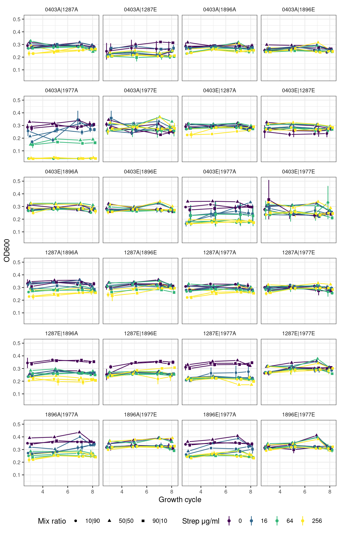
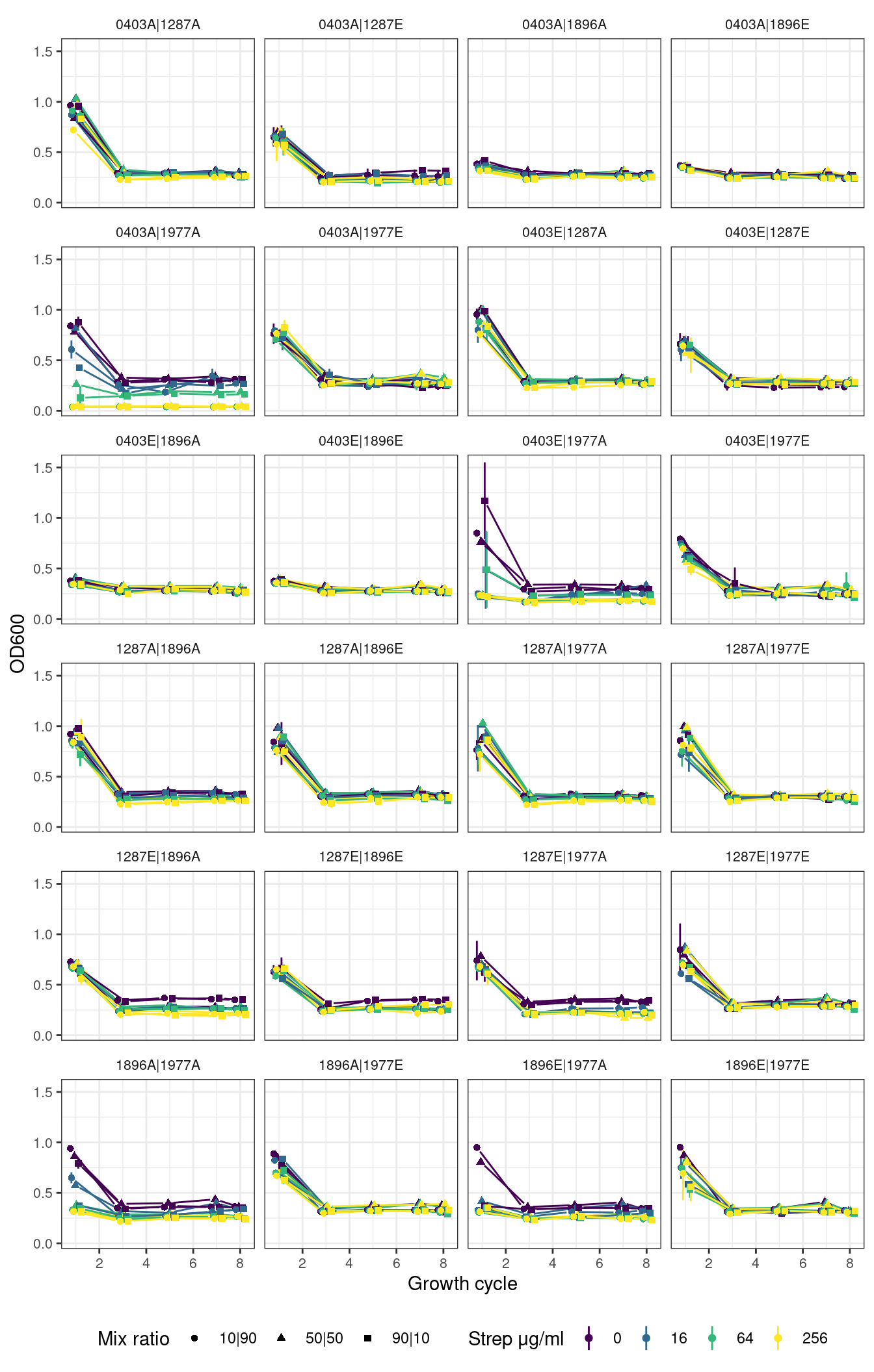
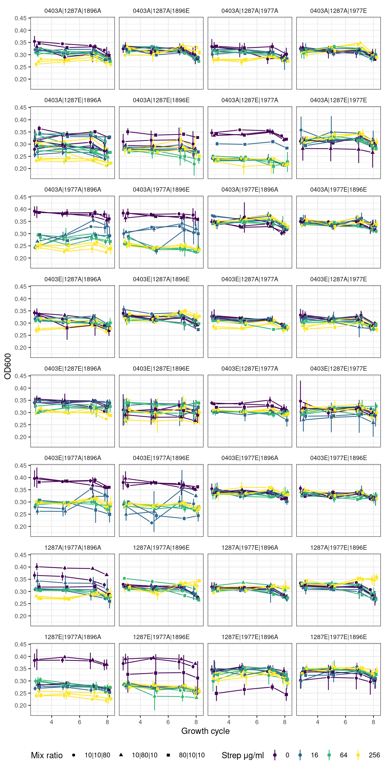
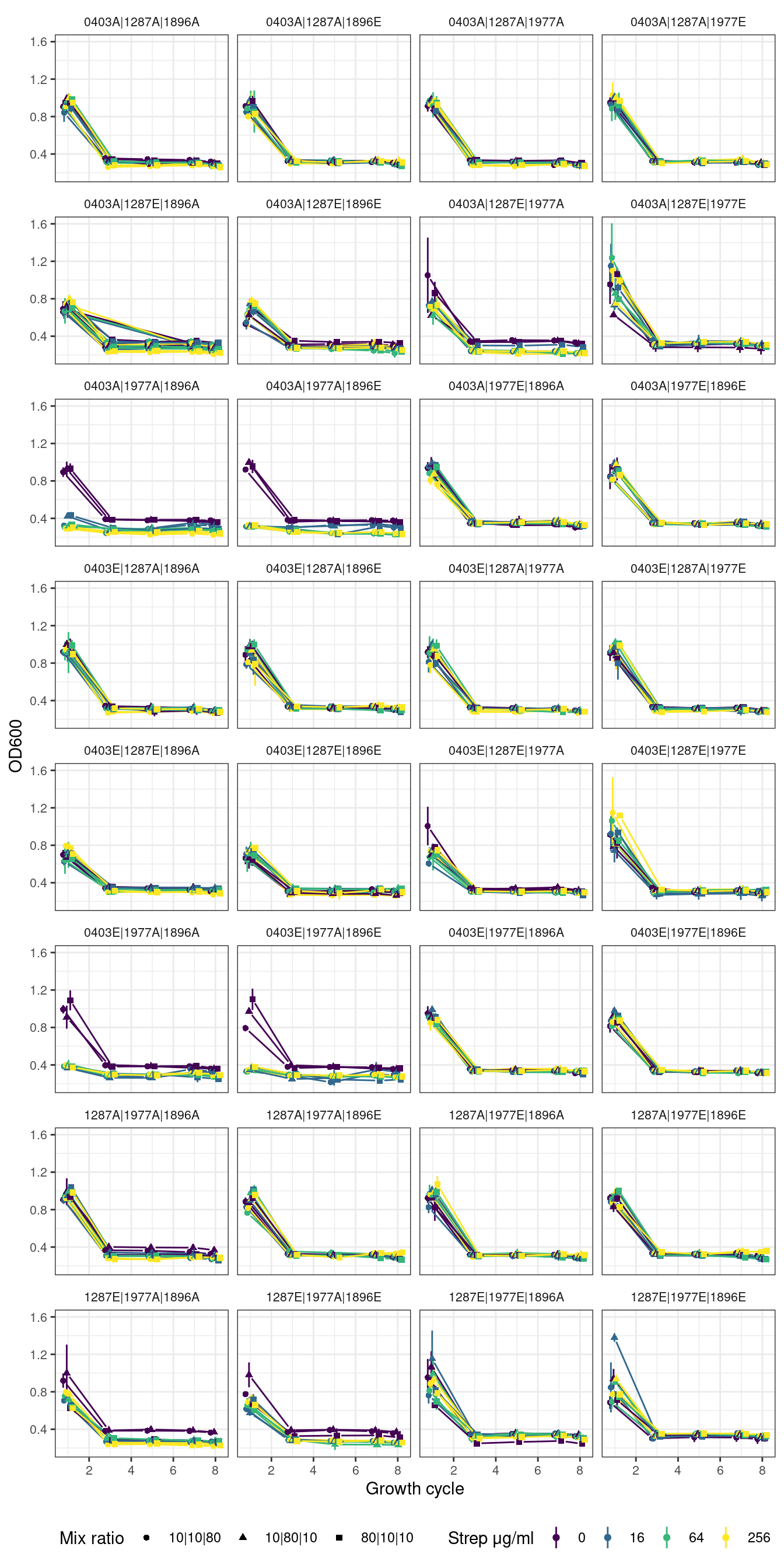
Here we will plot optical density over the batch growth cycles. For ease of visualization we exclude the first transfer because the OD was very high, and this happened in all conditions. We focus on the subsequent transfers because the OD has mostly stabilized after the first growth cycle.

2.1 Plotting functions

plot_od_grid <- function(df, remove_first_cycle = TRUE, ncol){
  pj <- ggplot2::position_jitterdodge(jitter.width=0.0,
                           jitter.height = 0.0,
                           dodge.width = 0.5,
                           seed=9)
  
  df %>% 
    dplyr::filter(if(remove_first_cycle) transfers > 2 else transfers > 0) %>%
    ggplot2::ggplot(aes(x = transfers, y = OD_mn, color = strep_conc, group = interaction(strep_conc, fr))) + 
    ggplot2::geom_linerange(aes(ymin = OD_mn - OD_sd, ymax = OD_mn + OD_sd, color = strep_conc), position = pj) + 
    ggh4x::geom_pointpath(aes(shape = fr), position = pj, mult = 0.2) +
    #ggplot2::geom_point() + 
    #ggplot2::geom_line(aes(linetype = f)) + 
    ggplot2::facet_wrap(~sp, ncol = ncol) +
    ggplot2::labs(x = "Growth cycle", y = "OD600", color = "Strep μg/ml", shape = "Mix ratio") +
    ggplot2::scale_color_viridis_d() +
    ggplot2::theme_bw() + 
    ggplot2::theme(strip.background = element_blank(),
        legend.position = "bottom", 
        axis.text = element_text(size = 8),
        strip.text = element_text(size = 8))
}

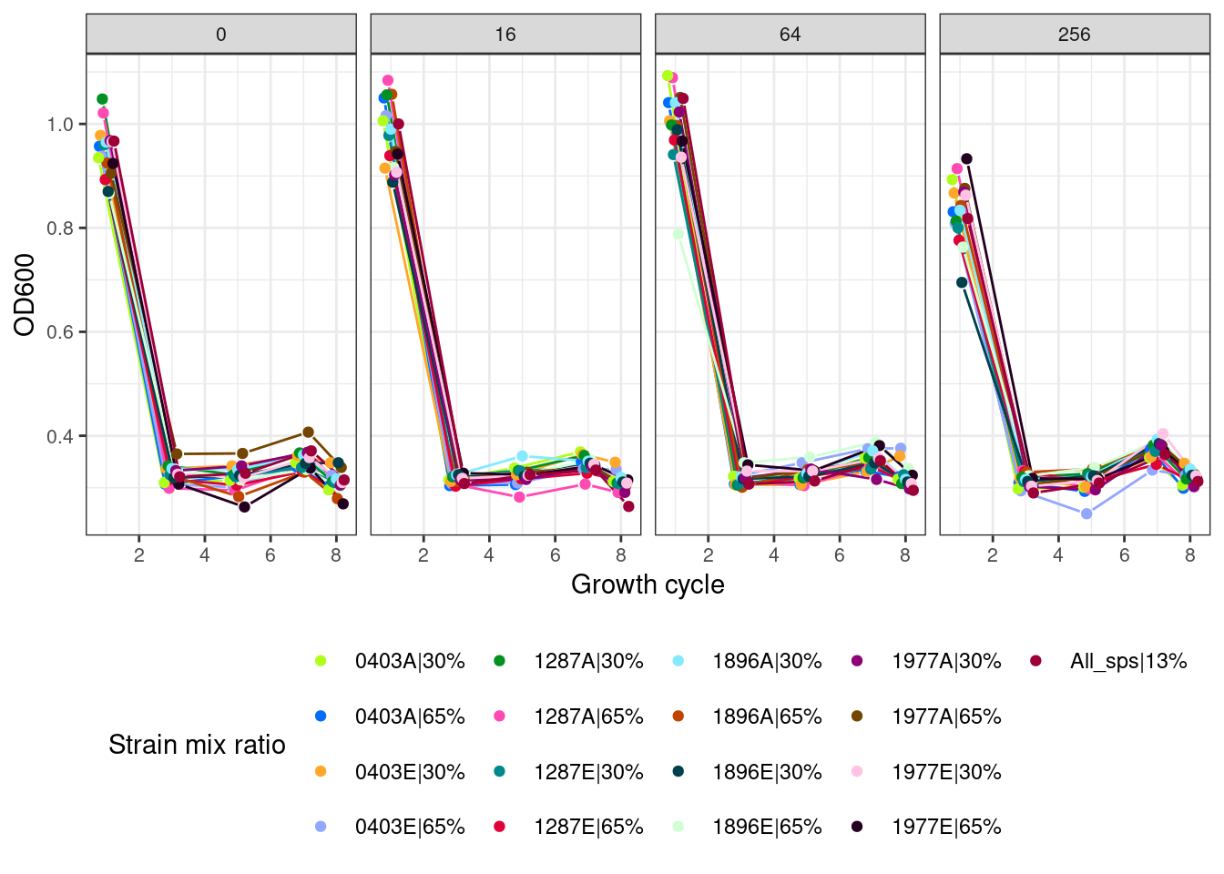
# Special Octets plotting function
plot_od_octets <- function(df, remove_first_cycle = TRUE, ncol){
  cols <- c("#b0fe1b","#006dff","#ffa728","#93a7ff",
          "#009121","#ff4ab4","#00898b","#e20039",
          "#85eaff","#bf4400","#003f4c","#d0ffd3",
          "#8d0077","#744500","#ffc3e3","#230020",
          "#9d0038")

  pj <- ggplot2::position_jitterdodge(jitter.width=0.0,
                           jitter.height = 0.0,
                           dodge.width = 0.5,
                           seed=9)

  df %>% 
    dplyr::filter(if(remove_first_cycle) transfers > 2 else transfers > 0) %>%
    ggplot2::ggplot(aes(x = transfers, y = OD, color = name, group = interaction(strep_conc, name))) + 
    ggh4x::geom_pointpath(position = pj, mult = 0.2) +
    ggplot2::facet_wrap(~strep_conc, ncol = ncol) +
    ggplot2::labs(x = "Growth cycle", y = "OD600", color = "Strain mix ratio") +
    ggplot2::scale_colour_manual(values = cols) +
    ggplot2::theme_bw() + 
    ggplot2::theme(
      #strip.background = element_blank(),
      legend.position = "bottom", 
      axis.text = element_text(size = 8),
      strip.text = element_text(size = 8))
}

2.2 Pairs

fig_pairs <- plot_od_grid(pairs_combo_f, remove_first_cycle = TRUE, ncol = 4)

# ggsave(
#   here::here("figs", ".svg"),
#   fig01,
#   width = 7,
#   height = 12,
#   units = "in",
#   device = "svg"
# )
# 
# ggsave(
#   here::here("figs", ".png"),
#   fig01,
#   width = 7,
#   height = 12,
#   units = "in",
#   device = "png"
# )

2.2.1 Pairs without first growth cycle

Figure 1: Species pairs optical density (y-axis) over series of 48 hour growth cycles (x-axis, 16 days total). Different panels in the grid contain distinct species pairs (A = ancestral, E = strep evolved). Colors show Streptomycin concentration in μg/ml and point shape shows the initial mixing ratio of each species (in the same order as specie listed in each panel). Note that data from the first growth cycle (after 48 hours) is excluded for ease of viewing.

2.2.2 Pairs with first growth cycle

plot_od_grid(pairs_combo_f, remove_first_cycle = FALSE, ncol = 4)

Figure 2: As in Figure 1 but including data from the first growth cycle.

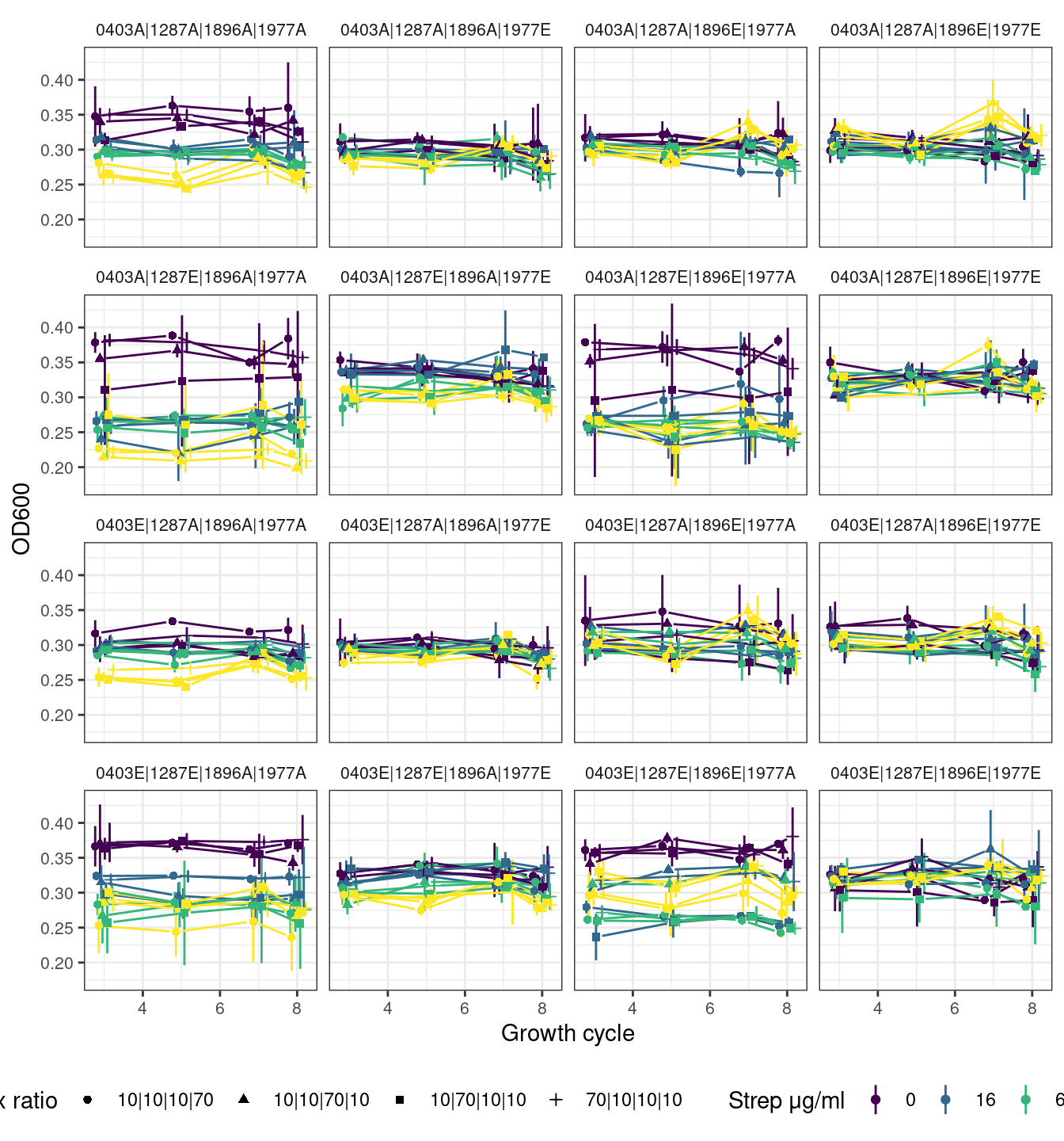
2.3 Trios

fig_trios <- plot_od_grid(trios_combo_f, remove_first_cycle = TRUE, ncol = 4)

# ggsave(
#   here::here("figs", ".svg"),
#   fig01,
#   width = 7,
#   height = 12,
#   units = "in",
#   device = "svg"
# )
# 
# ggsave(
#   here::here("figs", ".png"),
#   fig01,
#   width = 7,
#   height = 12,
#   units = "in",
#   device = "png"
# )

2.3.1 Trios without first growth cycle

Figure 3: Species trios optical density (y-axis) over series of 48 hour growth cycles (x-axis, 16 days total). Different panels in the grid contain distinct species pairs (A = ancestral, E = strep evolved). Colors show Streptomycin concentration in μg/ml and point shape shows the initial mixing ratio of each species (in the same order as species listed in each panel). Note that data from the first growth cycle (after 48 hours) is excluded for ease of viewing.

2.3.2 Trios with first growth cycle

plot_od_grid(trios_combo_f, remove_first_cycle = FALSE, ncol = 4)

Figure 4: As in Figure 3 but including data from the first growth cycle.

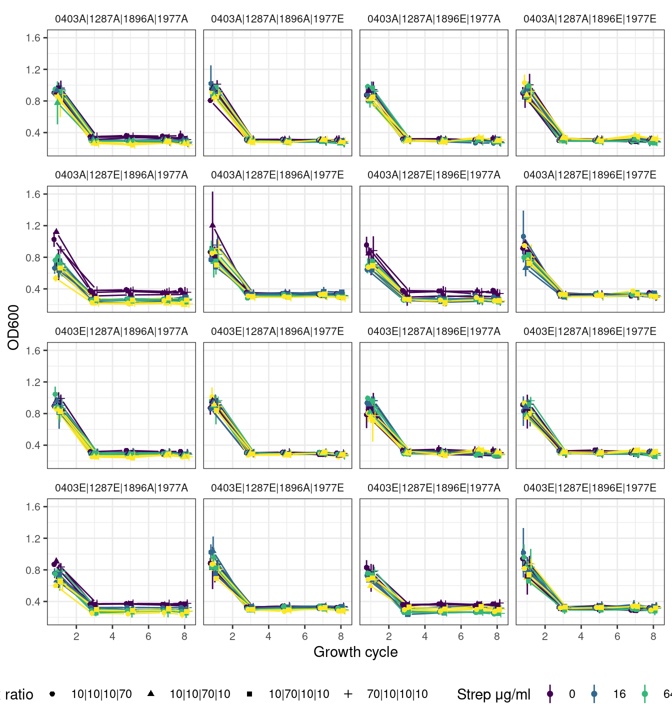
2.4 Quartets

fig_quarts <- plot_od_grid(quart_combo, remove_first_cycle = TRUE, ncol = 4)

# ggsave(
#   here::here("figs", ".svg"),
#   fig01,
#   width = 7,
#   height = 12,
#   units = "in",
#   device = "svg"
# )
# 
# ggsave(
#   here::here("figs", ".png"),
#   fig01,
#   width = 7,
#   height = 12,
#   units = "in",
#   device = "png"
# )

2.4.1 Quartets without first growth cycle

Figure 5: Species quartets optical density (y-axis) over series of 48 hour growth cycles (x-axis, 16 days total). Different panels in the grid contain distinct species pairs (A = ancestral, E = strep evolved). Colors show Streptomycin concentration in μg/ml and point shape shows the initial mixing ratio of each species (in the same order as species listed in each panel). Note that data from the first growth cycle (after 48 hours) is excluded for ease of viewing.

2.4.2 Quartets with first growth cycle

plot_od_grid(quart_combo, remove_first_cycle = FALSE, ncol = 4)

Figure 6: As in Figure 5 but including data from the first growth cycle.

2.5 Octets (all strains of all species)

2.5.1 Octets without first growth cycle

Figure 7: Strain octets (both evolved and ancestral forms added for all four species) optical density (y-axis) over a series of 48 hour growth cycles (x-axis, 16 days total). Different panels in the grid show the four different streptomycin treatments (0, 16, 64, and 256 ug/ml). Point colors represent the mix ratio of each strain. The strain listed is added at the listed percent and all other species are added at an equal ratio. Note that data from the first growth cycle (after 48 hours) is excluded for ease of viewing.

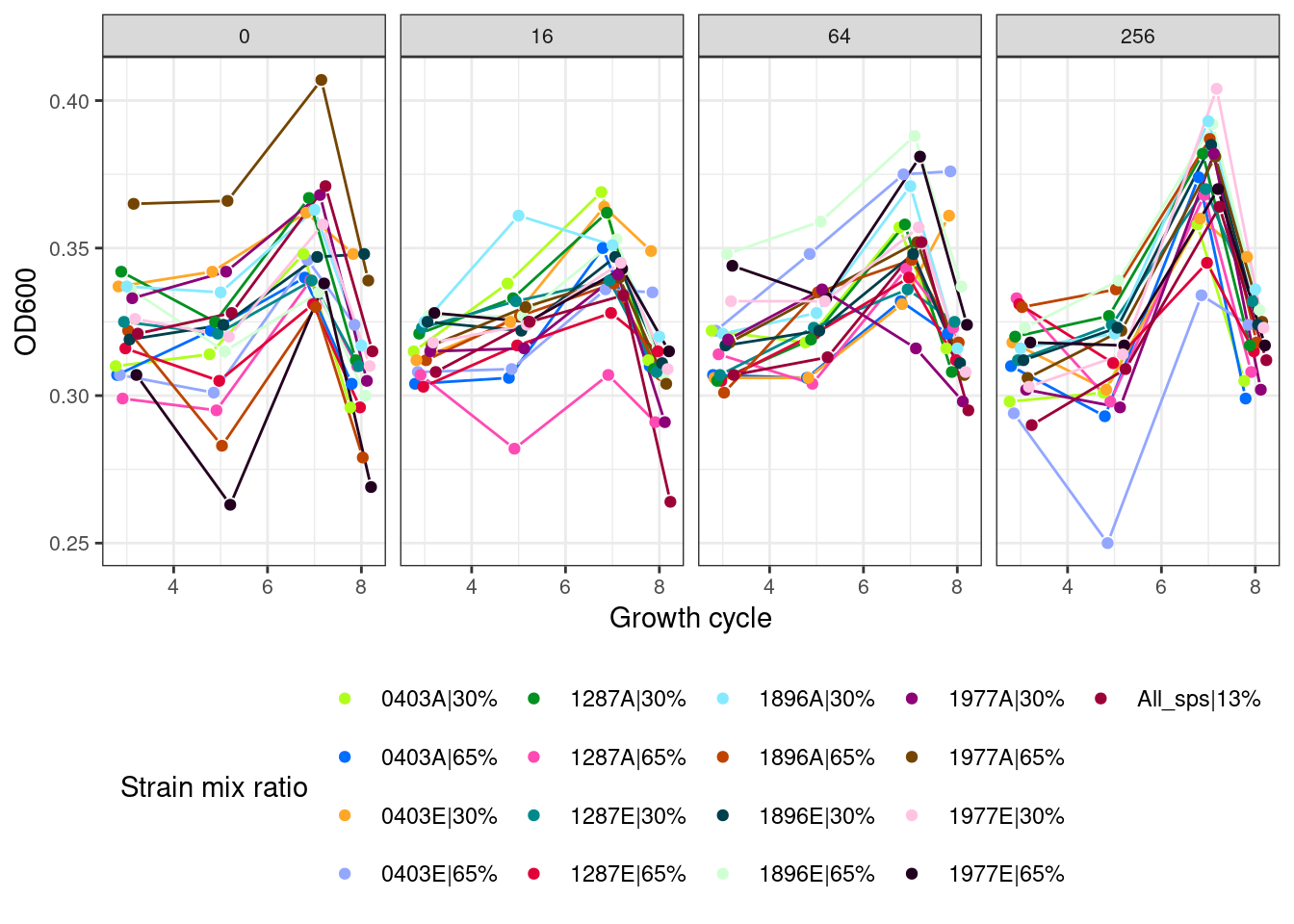
2.5.2 Octets with first growth cycle

Figure 8: As in Figure 7 but including data from the first growth cycle.