Violation of the pairwise assembly rule in 3 and 4-member communities
The pairwise asembly rule states “that in a multispecies competition, species that allcoexist with each other in pairs will survive, whereas species that are excluded by any of the surviving species will go extinct” (Friedman, 2017). Here we simply collect the competition outcomes from the pairwise experiments into a binary matrix, then we decompose the coexisting members (species with f > 1% | f < 99% after 8x 48 hour transfers) from each 3 or 4-member set into all unique constituent pairs, then we finally check whether those pairs coexist in in the pairwise binary matrix.
1 Setup
1.1 Libraries
1.2 Global variables
2 Read data
2.1 Pairwise coexistence outcomes
Rows: 95 Columns: 4
── Column specification ────────────────────────────────────────────────────────
Delimiter: "\t"
chr (2): sp_1, sp_2
dbl (2): strep_conc, coexists

ℹ Use `spec()` to retrieve the full column specification for this data.
ℹ Specify the column types or set `show_col_types = FALSE` to quiet this message.
Convert the pairs in tibble format into the matrixes
2.2 Species abundances
Show/hide code
samp_trios <- readr::read_tsv(here::here(data, "3sps_compiled.tsv")) %>%
  dplyr::rename(f = f_thresh) %>%
  dplyr::filter(community_type == "experiment") %>%
  dplyr::mutate(sp = paste(str_to_upper(evo_hist), str_extract(strainID, "\\d+"), sep = "_")) %>%
  dplyr::select(sample, strep_conc, replicate, n_species, sp, f, start_f=target_f_masterplate)

samp_quarts <- readr::read_tsv(here::here(data, "4sps_compiled.tsv")) %>%
  dplyr::rename(f = f_thresh) %>%
  dplyr::filter(community_type == "experiment") %>%
  dplyr::mutate(sp = paste(str_to_upper(evo_hist), str_extract(strainID, "\\d+"), sep = "_"))

samp_octs <- readr::read_tsv(here::here(data, "8sps_compiled.tsv")) %>%
  dplyr::rename(f = f_thresh) %>%
  dplyr::filter(community_type == "experiment") %>%
  mutate(target_f_masterplate = target_f_masterplate*100,
         max_f = max_f*100)
3 Trios: Application of the pairwise assembly rule
For species trios there are 32 different strain combinations. 4 all ancestral trios, 4 all evolved trios, and 24 trios containing a mixture of evolved and ancestral species
Show/hide code
samp_trios_fmt <- samp_trios %>%
  group_by(sample, strep_conc, replicate, n_species) %>%
  # for each sample create two new vars that record the species that went into
  # the trio and their rough relative abundance
  mutate(sp_set_id = paste(sp, collapse = ", "),
         sp_start_f = paste(start_f, collapse = ", ")) %>%
  # The next filter step ensures we remove species that went extinct and species
  # that were the only species left in the community (e.g., samples where 1287
  # was 100%) now we only look at species coexisting in each sample where there
  # are at least two species coexisting
  filter(f >= 0.01 & f <= 0.99) %>%
  # record as a variable a comma separated character of the rounded final
  # species abundances
  mutate(sp_final_f = paste(round(f, 2), collapse = ", ")) %>%
  # record a character variable of comma separated species that were found
  # coexisting at the final time point
  mutate(coexisting = paste(sp, collapse = ", ")) %>%
  ungroup() %>%
  dplyr::select(sample, strep_conc, replicate, n_species, sp_set_id, sp_start_f, sp_final_f, coexisting) %>%
  # removes redundant rows
  distinct() %>%
  # now use nest and strsplit so that we can record a character vector of coexisting species
  nest(.by = c(sample, strep_conc, replicate)) %>%
  mutate(coexisting = map(data, ~ strsplit(.x$coexisting, split=", ", fixed=TRUE)[[1]])) %>%
  #mutate(sp_set_id = map(data, ~strsplit(.x$sp_set_id, split=", ", fixed=TRUE)[[1]])) %>%
  # join with the pairwise coexistence matrixes
  left_join(pairs_matrixified, by = join_by(strep_conc))
Apply the coexistence rule test
There are 922 trio samples total
Show/hide code
291 Trio samples (291/922 = 31%) have at least 1 species pair combination that is inconsistent with outcomes from pairwise competition
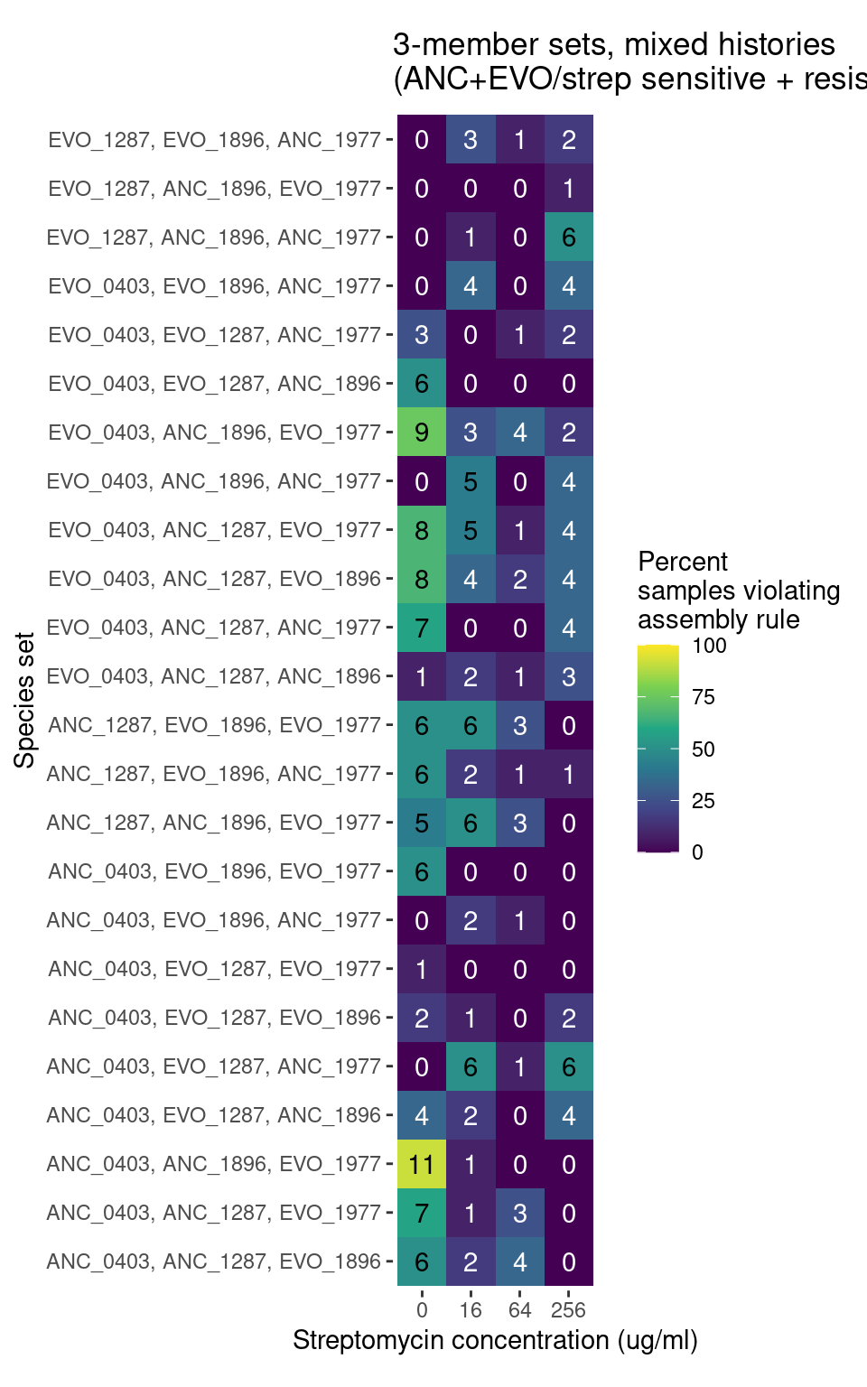
We can compare the distribution of these violations across different antibiotics levels and evolutionary histories
Show/hide code
# number of discrete samples with varying species starting frequencies for
# each species/strain combination
nreps <- 12

full_set <- samp_trios_ruletest_reduced %>%
  distinct(strep_conc, sp_set_id) %>%
  complete(sp_set_id, strep_conc)

samp_trios_ruletest_reduced_summary <- samp_trios_ruletest_reduced %>%
  filter(pair_coexists_alone == 0) %>%
  distinct(sample, strep_conc, replicate, n_species, sp_set_id) %>%
  group_by(strep_conc, sp_set_id) %>%
  count(name = "n_trios_w_pair_violation") %>%
  right_join(full_set, by = join_by(strep_conc, sp_set_id)) %>%
  replace_na(list(n_trios_w_pair_violation = 0)) %>%
  ungroup() %>%
  mutate(perc = n_trios_w_pair_violation/nreps*100,
         strep_conc = factor(strep_conc)) %>%
  mutate(evo_combo = case_when(str_detect(sp_set_id, "ANC") & str_detect(sp_set_id, "EVO") ~ "mix",
                               str_detect(sp_set_id, "ANC") &! str_detect(sp_set_id, "EVO") ~ "all_anc",
                               str_detect(sp_set_id, "EVO") &! str_detect(sp_set_id, "ANC") ~ "all_evo"))
Show/hide code
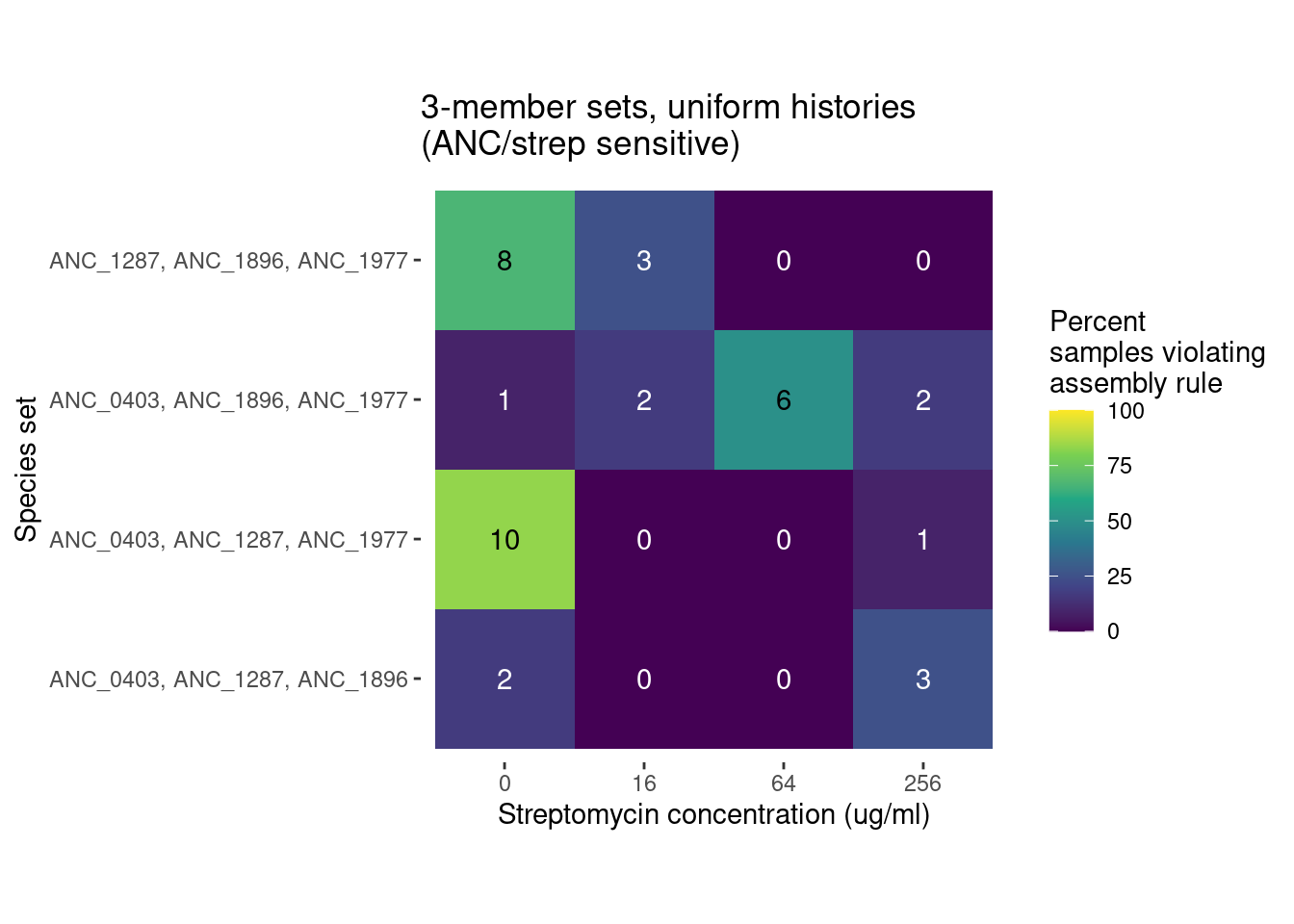
Show/hide code
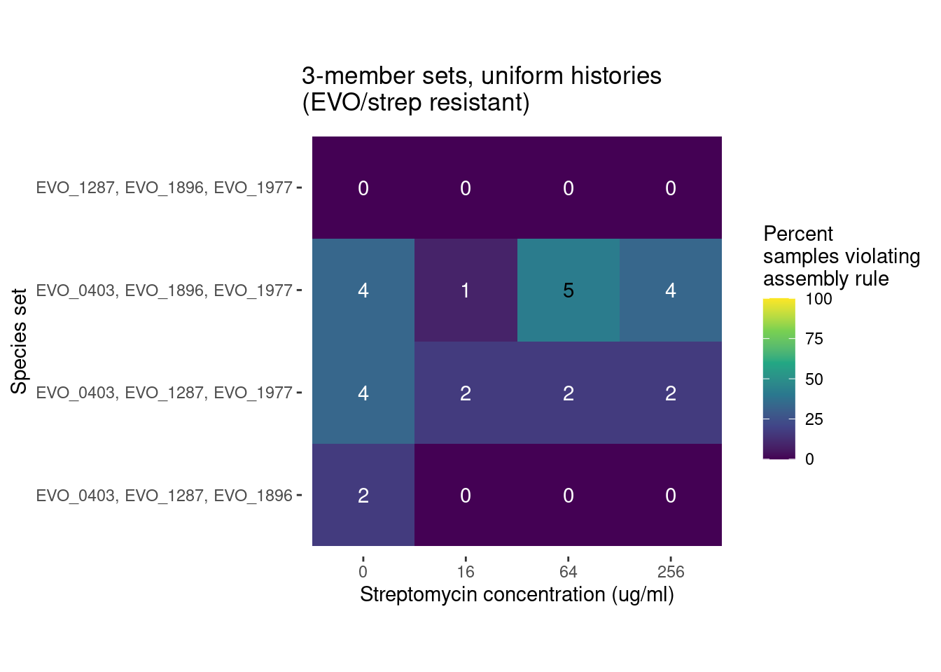
Show/hide code
Quick check into relative fraction of each grouping (all sensitive, all resistant, mixed sensitive/resistant) with at least one violation to the asse
Show/hide code
a <- samp_trios_ruletest_reduced_summary %>%
  group_by(strep_conc, evo_combo) %>%
  count(name = "ntot")

b <- samp_trios_ruletest_reduced_summary %>%
  group_by(strep_conc, evo_combo) %>%
  count(n_trios_w_pair_violation != 0)

left_join(b, a, by = join_by(strep_conc, evo_combo)) %>%
  mutate(f = n/ntot) %>%
  ggplot() +
  geom_col(aes(x = strep_conc, y = f, fill = `n_trios_w_pair_violation != 0`)) +
  facet_grid(~ evo_combo) +
  scale_x_discrete(guide = guide_axis(angle = 0)) +
  scale_y_continuous(labels = label_percent()) +
  labs(x = "Streptomycin concentration (ug/ml)", y = "Percentage of trio sets",
fill = "At least one experiment\nviolating assembly rule") 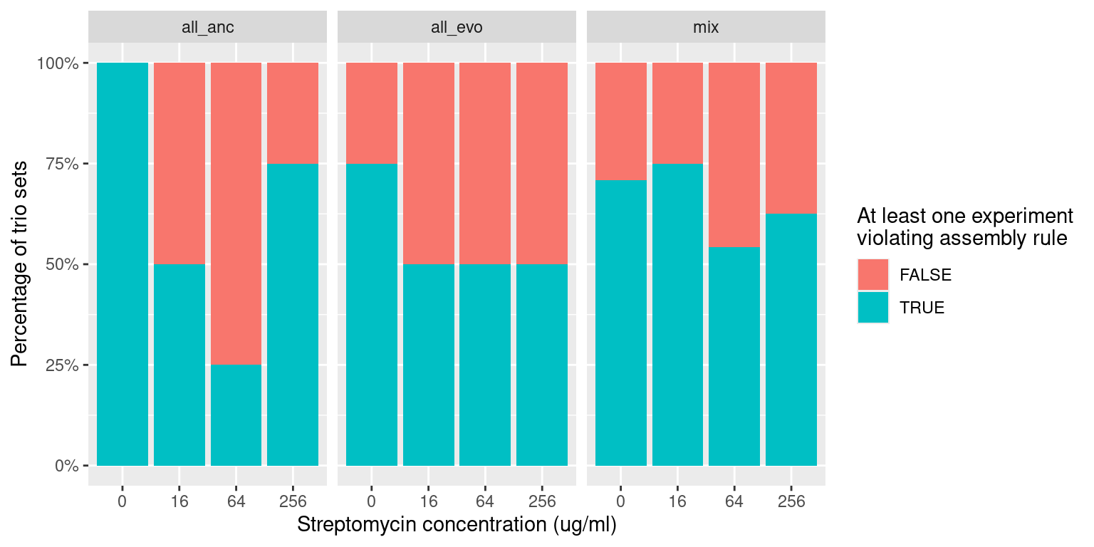
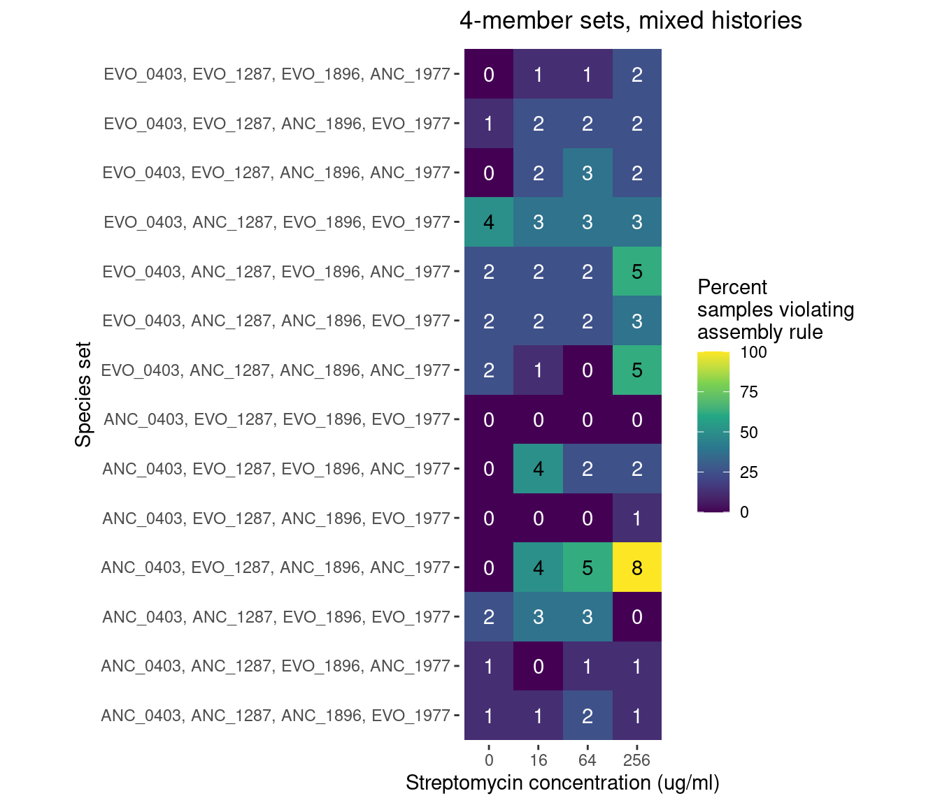
4 Quartets: Application of the pairwise assembly rule
For species quartets there are 16 different strain combinations. 1 all ancestral, 1 all evolved, and 14 containing a mixture of evolved and ancestral
Show/hide code
samp_quarts_fmt <- samp_quarts %>%
  group_by(sample, strep_conc, replicate, n_species) %>%
  # for each sample create two new vars that record the species that went into
  # the trio and their rough relative abundance
  mutate(sp_set_id = paste(sp, collapse = ", "),
         sp_start_f = paste(target_f_masterplate, collapse = ", ")) %>%
  # The next filter step ensures we remove species that went extinct and species
  # that were the only species left in the community (e.g., samples where 1287
  # was 100%) now we only look at species coexisting in each sample where there
  # are at least two species coexisting
  filter(f >= 0.01 & f <= 0.99) %>%
  # record as a variable a comma separated character of the rounded final
  # species abundances
  mutate(sp_final_f = paste(round(f, 2), collapse = ", ")) %>%
  # record a character variable of comma separated species that were found
  # coexisting at the final time point
  mutate(coexisting = paste(sp, collapse = ", ")) %>%
  ungroup() %>%
  dplyr::select(sample, strep_conc, replicate, n_species, sp_set_id, sp_start_f, sp_final_f, coexisting) %>%
  # removes redundant rows
  distinct() %>%
  # now use nest and strsplit so that we can record a character vector of coexisting species
  nest(.by = c(sample, strep_conc, replicate)) %>%
  mutate(coexisting = map(data, ~ strsplit(.x$coexisting, split=", ", fixed=TRUE)[[1]])) %>%
  # join with the pairwise coexistence matrixes
  left_join(pairs_matrixified, by = join_by(strep_conc))
Apply the coexistence rule test
Show/hide code
There are 512 quartet samples total
Show/hide code
116 Trio samples (116/512 = 23%) have at least 1 species pair combination that is inconsistent with outcomes from pairwise competition
We can compare the distribution of these violations across different antibiotics levels and evolutionary histories
Show/hide code
# number of discrete samples with varying species starting frequencies for
# each species/strain combination
nreps <- 8

full_set <- samp_quarts_ruletest_reduced %>%
  distinct(strep_conc, sp_set_id) %>%
  complete(sp_set_id, strep_conc)

samp_quarts_ruletest_reduced_summary <- samp_quarts_ruletest_reduced %>%
  filter(pair_coexists_alone == 0) %>%
  distinct(sample, strep_conc, replicate, n_species, sp_set_id) %>%
  group_by(strep_conc, sp_set_id) %>%
  count(name = "n_quarts_w_pair_violation") %>%
  right_join(full_set, by = join_by(strep_conc, sp_set_id)) %>%
  replace_na(list(n_quarts_w_pair_violation = 0)) %>%
  ungroup() %>%
  mutate(perc = round(n_quarts_w_pair_violation/nreps*100),
         strep_conc = factor(strep_conc)) %>%
  mutate(evo_combo = case_when(str_detect(sp_set_id, "ANC") & str_detect(sp_set_id, "EVO") ~ "mix",
                               str_detect(sp_set_id, "ANC") &! str_detect(sp_set_id, "EVO") ~ "all_anc",
                               str_detect(sp_set_id, "EVO") &! str_detect(sp_set_id, "ANC") ~ "all_evo"))
Show/hide code

Show/hide code
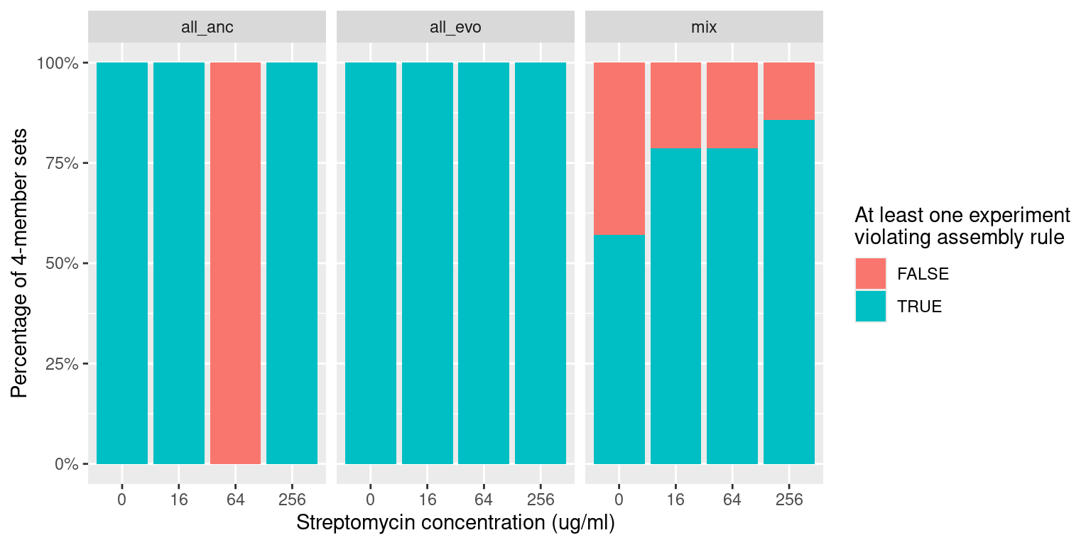
Quick check into relative fraction of each grouping (all sensitive, all resistant, mixed sensitive/resistant) with at least one violation to the asse
Show/hide code
a <- samp_quarts_ruletest_reduced_summary %>%
  group_by(strep_conc, evo_combo) %>%
  count(name = "ntot")

b <- samp_quarts_ruletest_reduced_summary %>%
  group_by(strep_conc, evo_combo) %>%
  count(n_quarts_w_pair_violation != 0)

left_join(b, a, by = join_by(strep_conc, evo_combo)) %>%
  mutate(f = n/ntot) %>%
  ggplot() +
  geom_col(aes(x = strep_conc, y = f, fill = `n_quarts_w_pair_violation != 0`)) +
  facet_grid(~ evo_combo) +
  scale_x_discrete(guide = guide_axis(angle = 0)) +
  scale_y_continuous(labels = label_percent()) +
  labs(x = "Streptomycin concentration (ug/ml)", y = "Percentage of 4-member sets",
       fill = "At least one experiment\nviolating assembly rule")